Intelligent Agents & Problem Formulation
The foundations of modern artificial intelligence and machine learning trace back to World War II. British mathematician and computer scientist Alan Turing and his team at Bletchley Park worked to crack the German military cipher machine, the Enigma. Turing and his colleagues engineered the electromechanical Bombe machine to systematically evaluate permutation spaces and decipher encrypted Axis communications. By demonstrating that mechanical automation could detect subtle statistical regularities in vast data spaces, the Enigma and Bombe machines established the conceptual bedrock of Machine Learning.
The earliest recognized work in artificial intelligence was published in 1943 by neurophysiologist Warren McCulloch and logician Walter Pitts. Their pioneering work synthesized three foundational disciplines:
- Physiology & Neuroanatomy: The biological structure, threshold firing, and synaptic behavior of neurons in the brain.
- Formal Propositional Logic: The formal axiomatic propositional calculus of Bertrand Russell and Alfred North Whitehead.
- Turing's Theory of Computation: Alan Turing's notion of universal computing machines and formal computability.
- Artificial Neuron Model: They proposed an idealized model of artificial neurons where each unit is binary—characterized as either ON (1 / firing) or OFF (0 / quiescent) based on whether incoming inputs exceed a fixed activation threshold.
- Universal Computability: They proved mathematically that any computable logical or arithmetic function could be computed by a suitably connected network of threshold neurons (implementing AND, OR, NOT operations).
- Capacity to Learn: They explicitly suggested that suitably defined networks can adapt their connection weights dynamically to learn from experience.
The Turing Test (1950): In his landmark paper "Computing Machinery and Intelligence", Alan Turing formulated an operational test for intelligence (the "Imitation Game"). Rather than debating the metaphysical question "Can machines think?", Turing proposed an empirical benchmark: A human interrogator submits written questions through a terminal to a hidden human and a hidden machine. If the interrogator cannot reliably distinguish the computer's answers from the human's, the computer passes the test as exhibiting human-level intelligence.
1950: The SNARC (The First Neural Network Computer): That same year, Marvin Minsky and Dean Edmonds at Harvard University engineered the world's first hardware neural network computer, named The SNARC (Stochastic Neural Analog Reinforcement Calculator). Built from 3,000 vacuum tubes, surplus B-24 bomber gyro-autopilots, and motor-driven potentiometers, it simulated a network of 40 synapses that learned to navigate a simulated maze via reinforcement principles.
The formal academic discipline of Artificial Intelligence was born in 1956 at the historic Dartmouth Summer Research Project on Artificial Intelligence, organized by John McCarthy (then at Dartmouth College), Marvin Minsky, Nathaniel Rochester, and Claude Shannon. McCarthy coined the term "Artificial Intelligence" and is universally recognized as the "Father of AI".
- In 1958, McCarthy invented LISP (List Processing), which remained the preeminent programming language for AI for more than three decades.
- The period between 1952 and 1969 witnessed intense discovery, including Arthur Samuel's self-learning Checkers program, the Logic Theorist, and early natural language parsers (ELIZA).
| Historical Era | Key Characteristics & Technological Drivers | Societal & Economic Impact |
|---|---|---|
| 1950s–1960s: First AI Boom |
Symbolic reasoning, search trees, prototype neural models (Perceptrons), and early heuristic problem-solving programs. | Unprecedented academic enthusiasm and generous defense/government funding (DARPA). |
| 1974–1980: First AI Winter (Slide 11) |
Researchers failed to materialize promised results (e.g. automated Russian-to-English translation failed due to lack of real-world context; Minsky & Papert proved Perceptrons could not solve XOR). | Subjected to severe academic criticism; major funding cuts (Lighthill Report in the UK, Mansfield Amendment in the US). |
| 1980–1987: Second AI Boom (Slide 12) |
Widespread corporate adoption of Expert Systems—programs solving high-value domain problems using rule-based inference engines (\(\text{IF-THEN}\) logic) capturing human expert knowledge (e.g., XCON at DEC, MYCIN in medical diagnosis). | Over a billion dollars invested by commercial enterprises into specialized AI workstations and LISP machines. |
| 1987–1993: Second AI Winter |
Expert system knowledge bases proved brittle and extraordinarily expensive to maintain; desktop PCs (Apple, IBM) overtook specialized LISP hardware. | Collapse of the specialized LISP hardware market; widespread corporate disillusionment. |
| Year | Milestone Achievement | Significance to AI & Computer Science |
|---|---|---|
| 1997 (Slide 13) | IBM Deep Blue defeats World Chess Champion Garry Kasparov in a 6-game match (3.5–2.5). | First time a reigning world chess champion was defeated by a computer under tournament conditions. Demonstrated the immense power of custom parallel hardware, alpha-beta tree search, and specialized evaluation functions. |
| 2005 (Slide 14) | Stanley, the autonomous vehicle developed by Stanford University, wins the DARPA Grand Challenge. | Successfully navigated 132 miles of rough, unpaved Mojave desert terrain without human intervention using machine vision, probabilistic laser mapping (LIDAR), and reinforcement control. |
| 2011 (Slide 15) | IBM Watson defeats former champions Ken Jennings and Brad Rutter on Jeopardy! | Showcased advanced Natural Language Processing, entity extraction, and automated reasoning over massive unstructured encyclopedic corpora under strict real-time buzzer latency. |
| 2015 (Slide 16) | Deep Convolutional Neural Networks (ResNet, VGGNet, GoogLeNet) dominate the ImageNet Competition. | Deep learning reduced image classification top-5 error rates to 3.6%, officially surpassing the human benchmark (~5.0%) and igniting the modern deep learning revolution. |
| 2016 (Slide 17) | Google DeepMind's AlphaGo defeats 18-time world Go champion Lee Sedol (4–1). | Go possesses a branching factor of ~250 and \(10^{170}\) states (exceeding atoms in the universe). Solved using Deep Reinforcement Learning, Value Networks, Policy Networks, and Monte Carlo Tree Search. |
| 2018 (Slide 18) | OpenAI releases GPT (Generative Pre-trained Transformer). | Demonstrated that self-supervised pre-training on large internet text corpora followed by fine-tuning yields unprecedented general language generation, translation, and comprehension capabilities. |
Machine Learning (ML) is the primary sub-field of AI driving modern applications. Rather than hand-coding static rules, ML algorithms get smarter and improve their predictive accuracy the more data they are given. By ingesting large training datasets, the system identifies latent mathematical patterns and formulates generalizable decision rules.
| Learning Paradigm | Dataset Nature | Core Mechanism & Objective | Lecture Slide Example |
|---|---|---|---|
| 1. Unsupervised Learning (Slide 24) | Unlabelled Data (no predefined target outcomes or teacher signals). | The algorithm analyzes raw data to discover inherent structures, density groupings, or geometric clusters without prior knowledge. | Fruit & Vegetable Sorting: A raw basket of mixed onions, eggplants, bell peppers, and tomatoes is automatically clustered into distinct groups based purely on visual similarities (color, shape, size). |
| 2. Supervised Learning (Slide 25) | Labelled Dataset (each input vector \(X\) is paired with a known ground-truth label \(Y\)). | The model infers a mapping function \(f: X \to Y\). During training, prediction errors adjust weights so the model accurately classifies unseen test data. | Agricultural Produce Classifier: The model is fed thousands of labeled images: [Image of Carrot \(\to\) "Carrot"], [Image of Bell Pepper \(\to\) "Bell Pepper"], [Image of Tomato \(\to\) "Tomato"]. Given a new image, it correctly outputs "Bell Pepper". |
| 3. Semi-Supervised Learning (Slide 26) | Small amount of labelled data combined with a large volume of unlabelled data. | Acquiring manual labels is expensive and time-consuming. The model uses the few labeled examples to establish anchor classes and leverages the geometry of unlabeled data to refine the decision boundary. | Fruit Recognition with Incomplete Labels: You have only 2 labeled images ("Banana", "Apple") and thousands of unlabeled images of bananas, apples, and grapes. The model clusters the dataset and predicts labels for the unlabeled clusters accurately. |
| 4. Reinforcement Learning (Slide 27) | Trial-and-error interactions with an external dynamic Environment. | The Agent observes the current State, executes an Action, and the Environment transitions to a new state and returns a scalar Reward or Penalty feedback. The objective is to learn an optimal policy \(\pi(s)\) that maximizes cumulative rewards over time ("learning by doing"). | Game Playing & Robotics: An autonomous navigation robot or chess agent makes moves. Winning or navigating safely grants positive rewards (+10), while collisions or losing pieces deliver penalties (-50). Over thousands of iterations, it discovers optimal move sequences. |
Artificial Neural Networks (ANNs) were mathematically engineered to mimic the human brain's pattern recognition and distributed decision-making capabilities. Below is the precise anatomical and computational mapping:
    BIOLOGICAL NEURON ANATOMY               ARTIFICIAL NEURON (PERCEPTRON)
    ─────────────────────────               ──────────────────────────────
    Dendrites (Input branches)      ───►    Input Features: \(x_1, x_2, \dots, x_n\)
    Synaptic Gaps / Strengths       ───►    Synaptic Weights: \(w_1, w_2, \dots, w_n\)
    Soma (Cell Body / Nucleus)      ───►    Summation Junction: \(\sum (w_i x_i) + \text{Bias } b\)
    Action Potential Threshold      ───►    Activation Function: \(\sigma(z)\) (e.g. Step, ReLU, Sigmoid)
    Axon (Transmission Line)        ───►    Axonal Signal Conduction
    Axon Terminals / Synapses       ───►    Output Activation: \(y = \sigma\left(\sum w_i x_i + b\right)\)
Biological Structure: Comprises the Dendrite (receives electrochemical neurotransmitters), Soma (integrates signals), Nucleus, Axon (long electrical transmission fiber), Schwann Cells & Myelin Sheath (insulate the axon to accelerate impulse conduction), Node of Ranvier (periodic unmyelinated gaps where the action potential regenerates), and Axon Terminal (transmits signals to adjacent neurons).
Artificial Network: Arranged in an Input Layer (raw feature inputs), one or more Hidden Layers (hierarchical feature extractors learning non-linear abstractions), and an Output Layer (final classification or continuous value regression).
Natural Language Processing (NLP) is the branch of AI dedicated to programming computers to process, understand, interpret, and generate human languages to facilitate natural interaction between humans and machines.
The Core Challenge of NLP: Human language is inherently unstructured, highly ambiguous, context-dependent, and governed by complex linguistic rules. NLP leverages mathematical algorithms, grammatical formalisms, and neural models to recognize and abstract the latent rules of natural languages, converting unstructured speech and text into a structured, computer-understandable representation.
- IVR (Interactive Voice Response): Automated voice telephony systems used in customer support call centers to understand spoken customer queries and route calls intelligently.
- Machine Translation: Cross-lingual translation systems like Google Translate and DeepL that translate text between hundreds of global languages.
- Syntax & Grammar Assistants: Tools like Grammarly and Microsoft Word spell-checkers that analyze grammatical syntax and stylistic phrasing in real-time.
- Virtual Assistants & Conversational Chatbots: Conversational agents such as Apple Siri, Google Assistant, Amazon Alexa, and Large Language Model assistants (ChatGPT) that execute voice tasks and converse seamlessly with users.
To fully process human communication, modern NLP systems execute five hierarchical analytical stages:
   ┌──────────────────┐      ┌──────────────────┐      ┌──────────────────┐
   │ Lexical Analysis │ ───► │Syntactic Analysis│ ───► │ Semantic Analysis│
   │ (Tokenization)   │      │(Grammar Parsing) │      │ (Literal Meaning)│
   └──────────────────┘      └──────────────────┘      └────────┬─────────┘
                                                                │
   ┌──────────────────┐      ┌──────────────────┐               │
   │    Discourse     │ ◄─── │Pragmatic Analysis│ ◄─────────────┘
   │   Integration    │      │(Hidden Intent &  │
   │ (Context Links)  │      │ Situational Role)│
   └──────────────────┘      └──────────────────┘
| NLP Stage | Formal Linguistic Mechanism | Intuition & Real-World Course Slide Examples |
|---|---|---|
| 1. Lexical Analysis / Integration (Slide 30) | Converts a continuous stream of raw characters or speech waves into discrete grammatical units called tokens. A lexer segments text into words, morphemes, prefixes, and punctuation marks. Often combined with a morphological parser. | "It's like cutting sentences into small pieces for better understanding." Input: "The train arrived." \(\to\) Tokens: ["The", "train", "arrived", "."]. |
| 2. Syntactic Analysis / Integration (Slide 30) | Analyzes the sequence of tokens conforming to formal grammar rules (e.g., Context-Free Grammars) to construct a hierarchical parse tree. Grammatical rules apply to categories and groups of words (Noun Phrases, Verb Phrases), not isolated words. | Checks if words follow grammar rules. Used in compilers, Grammarly, and Google Translate. Example: "The student writes code" \(\to\) Valid (Subject + Verb + Object). "Student code the writes" \(\to\) Syntax Error (violates word-order rules). |
| 3. Semantic Analysis / Integration (Slides 30–31) | Attempts to understand the true literal meaning of human language. It evaluates whether the logical structuring and semantic roles make sense in physical and domain reality. | Even if grammar is correct, does the meaning make sense in reality? • Sentence 1: "I deposited money in the bank." \(\implies\) \(\checkmark\) Valid semantic meaning.• Sentence 2: "I deposited fish in the bank." \(\implies\) \(\times\) Semantically anomalous / nonsensical in banking reality, despite having identical grammatical syntax! |
| 4. Pragmatic Analysis (Slide 31) | Discovers the hidden intent, communicative purpose, and real-world social context behind words beyond their literal semantic definition. | Understands the speaker's true intent based on situational context: • Utterance: "Can you open the window?"• Literal Semantic Analysis: An inquiry into whether the listener possesses the physical strength to slide the window pane. • Pragmatic Analysis: Identifies that this sentence is socially a polite request to open the window, requiring an action rather than a "Yes/No" answer! |
| 5. Discourse Integration (Slide 31) | Connects the current sentence with preceding conversational context to achieve coherent multi-turn comprehension (coreference resolution, anaphora resolution). | Links pronouns and contextual references across conversational turns: • Person 1: "I bought a new phone yesterday."• Person 2: "How much did it cost?"• Discourse Resolution: The pronoun "it" is immediately bound to the antecedent "new phone" by resolving the cross-sentence dialogue context. |
In classical AI taxonomy, intelligent systems are divided into four fundamental functional categories based on their internal cognition, memory retention, and consciousness:
| Category | Cognitive & Memory Capabilities | Primary Limitations | Course Slide Examples |
|---|---|---|---|
| 1. Reactive Machines (Slide 36) | The most fundamental form of AI. They perceive the current world state and react based on immediate condition-action rules. They possess no memory and cannot store or recall past experiences to influence future actions. | Cannot learn from mistakes or adapt to novel scenarios outside hardcoded evaluation heuristics. Identical inputs always produce identical outputs. | IBM Deep Blue: Evaluates chess pieces on the current board and selects the highest-scoring legal move, but possesses no memory of previous games or past moves made by the opponent. |
| 2. Limited Memory (Slide 37) | Can store past experiences and historical telemetry temporarily over a short time horizon to inform ongoing, real-time decisions. | Memory is transient and task-focused; it is not retained as long-term personal episodic experience or holistic autobiographical knowledge. | Self-Driving Cars (e.g., Tesla Autopilot, Waymo): Tracks the trajectory, speed, and acceleration of surrounding vehicles over the past several seconds to make safe lane changes, merge, and brake. |
| 3. Theory of Mind (Slide 38) | A more advanced AI paradigm (under active frontier research). These systems are designed to understand that humans and other agents possess their own emotions, thoughts, beliefs, mental states, and social intentions. | Extremely difficult due to the psychological complexity of human emotional states, social conventions, and subtle cultural cues. | Advanced Empathetic Personal Assistants & Social Robots: Companion systems that can sense when a human user is frustrated, grieving, or anxious, and adapt their tone, advice, and behavior accordingly. |
| 4. Self-Aware AI (Slide 39) | The theoretical ultimate pinnacle of AI (Artificial Superintelligence - ASI). These systems possess their own independent consciousness, self-awareness, inner feelings, desires, and subjective agency. | Strictly theoretical; does not currently exist. Entails profound philosophical, safety, existential, and alignment challenges. | Hypothetical sentient machines that are smarter, faster, and more intellectually capable than the biological human brain, possessing an intrinsic sense of self. |
Intelligence in general is defined as the "Ability to acquire and apply knowledge and skills". Our human species is biologically designated as Homo Sapiens: from Latin, Homo meaning "Man", and Sapiens meaning "Wise" or "Reasoning". Our survival and dominance as a species stem directly from our intellectual capacity.
For thousands of years, philosophers, psychologists, and biologists sought to understand how the human brain functions. The field of Artificial Intelligence goes far beyond passive cognitive psychology: AI not only attempts to understand how the brain functions, but actively engineers intelligent entities capable of autonomous decision-making.
There is no single universally accepted definition of Artificial Intelligence. In general, AI refers to the simulation of human intelligence processes by machines, especially computer systems. These simulated cognitive processes include learning (acquiring information and rules for using it), reasoning (using rules to reach conclusions), self-correction, and autonomous adaptation.
• Machine Learning (ML): Algorithms that allow machines to learn patterns and improve from experience without being explicitly programmed.
• Natural Language Processing (NLP): Systems that facilitate bidirectional interaction, understanding, and generation of human natural language.
• Computer Vision (Machine Vision): Algorithms that interpret, process, extract features, and understand visual data from photos, video streams, and multispectral sensors.
Artificial Intelligence refers to developing computer systems for performing tasks requiring human intelligence. These systems assess large volumes of data to identify complex patterns and make logical decisions. The ultimate goal of AI is to create machines to carry out diverse real-world tasks. The top 4 core techniques are:
| Technique (Slide 21) | Operational Mandate | Real-World Industrial Exemplar |
|---|---|---|
| 1. Machine Learning | Statistical optimization algorithms (Supervised, Unsupervised, RL) that extract patterns from training data to predict outcomes. | Fraud detection in banking, recommendation systems (Netflix, Spotify), predictive medical diagnostic classifiers. |
| 2. Natural Language Processing (NLP) | Computational linguistics and neural sequence models that convert unstructured human language into computer-understandable representations. | Google Translate, Siri, conversational chatbots, LLMs (ChatGPT, Gemini), interactive call center voice bots. |
| 3. Automation & Robotics | Cyber-physical hardware and sensory actuators engineered to execute precise mechanical tasks, navigation, and physical labor. | Automated factory assembly lines, Amazon warehouse sorting robots, surgical robotics (da Vinci), lunar rovers. |
| 4. Machine Vision | Image processing and deep convolutional neural networks that extract spatial patterns, classify visual scenes, and track objects. | Autonomous driving camera perception (Tesla Autopilot), biometric facial recognition, industrial assembly defect inspection. |
- Problem-Solving (Slide 32): AI solves complex problems that would normally demand human cognitive intelligence—spanning visual pattern recognition, speech parsing, multi-criteria decision making, and real-time language translation.
- Training via Big Data (Slide 33): AI models are not born capable; they are trained using massive empirical datasets. For example, speech recognition models are trained on hundreds of thousands of hours of acoustic spoken language recordings.
- Benefits of AI (Slide 35): (1) Vastly improves efficiency and industrial productivity, (2) Makes faster, objective, and data-informed decisions, (3) Performs hazardous tasks dangerous for human workers (bomb disposal, deep-sea exploration, toxic chemical handling), and (4) Drives frontier research in self-driving cars, voice assistants, and predictive healthcare.
What is State-of-the-Art (SOTA)? (Slide 64): The term represents the newest, most advanced, and most developed technology or method available today. Known as "cutting-edge" or "leading-edge" innovation, SOTA signifies the most modern, highest-performing version of a technology.
SOTA in AI (Slide 65): AI has been steadily evolving for over 70 years, not created overnight. SOTA AI refers specifically to: (1) The most advanced AI models, (2) The latest algorithmic techniques and architectures, and (3) The highest empirical performance and accuracy.
• ChatGPT / Foundation LLMs: Advanced natural language understanding, complex reasoning, and code generation.
• Tesla Autopilot / Waymo: Real-time vision-based autonomous driving and path planning.
• Google DeepMind AlphaFold: Revolutionary biological breakthrough predicting 3D protein structures with atomic accuracy.
• Medical AI: High-precision diagnostic systems detecting cancers, pneumonia, and retinal pathologies from X-rays and scans.
| The 4 Core Benefits of SOTA AI (Slide 67) | Industrial & Scientific Significance |
|---|---|
| 1. Higher Accuracy | Produces significantly better predictions, lower error rates, and superior diagnostic precision. |
| 2. Faster Processing | Accelerates complex decision-making from days of human analysis to milliseconds of compute. |
| 3. Competitive Advantage | Enables businesses and research institutions to outperform rivals and capture market leadership. |
| 4. Innovation Power | Unlocks entirely new scientific frontiers, novel drug designs, and technologies previously impossible. |

i. Simple Reflex Agent:
A Simple Reflex Agent is the most fundamental category of intelligent agents that selects actions strictly based on the current percept, completely ignoring the historical sequence of past percepts. It operates using condition-action rules (e.g., IF status == Dirty THEN action = Suck). It can only succeed in fully observable environments; if the environment is partially observable, it can suffer from infinite loops and thrashing behavior.
ii. The State of the Art (SOTA) in AI:
State-of-the-Art (SOTA) refers to the highest level of general technological development and performance achieved at a specific time. In modern AI, SOTA systems represent frontier capabilities across multiple domains, including:
- Large Language & Multimodal Foundation Models: Advanced reasoning and understanding systems like GPT-4o, Gemini 1.5/2.0 Pro, and Claude 3.5 Sonnet.
- Autonomous Physical Agents: Commercial Level-4 autonomous vehicles (Waymo, Tesla FSD) and humanoid robotics.
- Scientific Discovery: DeepMind's AlphaFold 3 (3D molecular biology and protein structure prediction).
- Superhuman Game Playing: AlphaGo, AlphaZero, and Stockfish NNUE exceeding all human grandmasters.
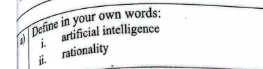
i. Artificial Intelligence (AI):
Artificial Intelligence is the branch of computer science dedicated to engineering computational systems that can perceive their environment, learn from experience, reason logically, and autonomously perform tasks that typically require human cognitive intelligence (such as decision-making, visual perception, and problem-solving).
ii. Rationality:
Rationality is the property of an agent acting to do the "right thing"—mathematically defined as selecting actions that maximize its expected performance measure given the percept sequence observed so far and its built-in domain knowledge. Rationality does not mean omniscience or perfection; it means optimal expected performance under uncertainty.
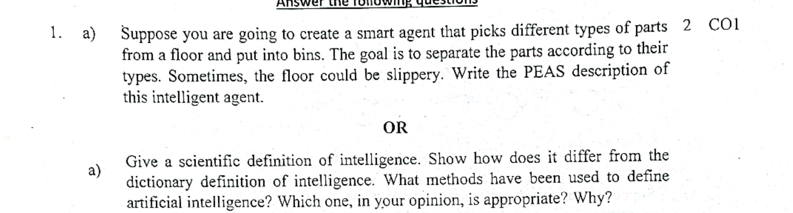
1. Scientific Definition of Intelligence vs. Dictionary Definition:
- Dictionary Definition: "The ability to acquire and apply knowledge and skills" (Oxford/Webster). This definition is human-centric, vague, and lacks quantifiable operational metrics for computational systems.
- Scientific Definition: A computational entity's capacity to perceive environmental states via sensors, construct internal world models, evaluate alternative candidate action sequences using expected utility, and execute actions via actuators to achieve specific goals under uncertainty and resource constraints.
2. Methods Used to Define Artificial Intelligence:
- Thinking Humanly: Cognitive modeling approach; reverse-engineering the neural and psychological workings of the human mind.
- Thinking Rationally: The "Laws of Thought" approach; formalizing deductive inference using mathematical logic (syllogisms, First-Order Logic).
- Acting Humanly: The Turing Test approach; evaluating whether a machine can converse indistinguishably from a human interrogator.
- Acting Rationally: The Rational Agent approach; building systems that act to achieve the best expected outcome based on their beliefs and percepts.
3. Which Definition is Most Appropriate and Why:
The Acting Rationally (Rational Agent) approach is universally recognized as the most appropriate standard in contemporary AI because:
- It is mathematically objective and quantifiable via expected utility theory.
- It is more general than human thought, as humans frequently behave irrationally due to emotional biases or cognitive limits.
- It facilitates rigorous engineering and algorithmic optimization (search, probabilistic reasoning, reinforcement learning).
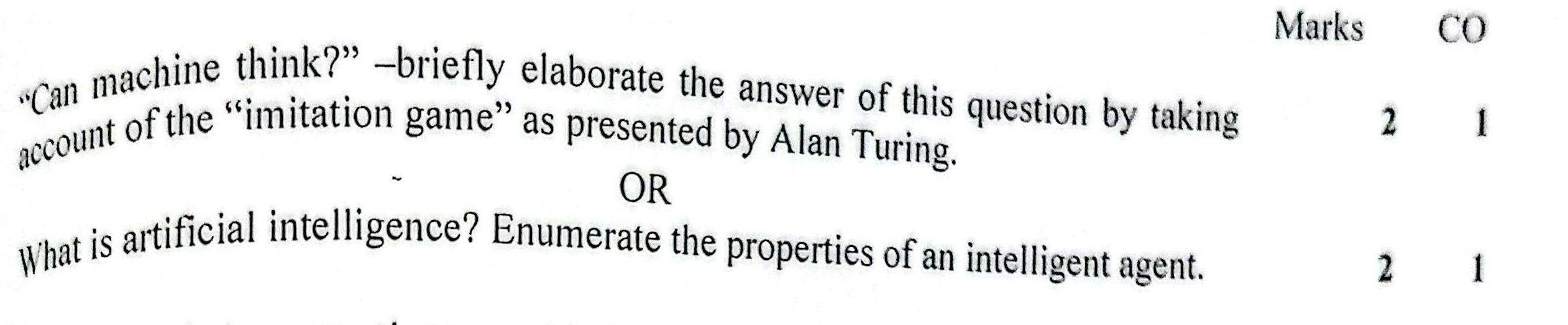
"Can machine think?" & Alan Turing's Imitation Game:
In his seminal 1950 paper Computing Machinery and Intelligence, British mathematician Alan Turing argued that the metaphysical question "Can machines think?" is too ambiguous. He proposed replacing it with an operational behavioral benchmark called the Imitation Game (The Turing Test):
- Setup: A human interrogator is situated in a separate room from two respondents: a human and a digital computer. Communication occurs solely via text terminals.
- Rule: The interrogator poses arbitrary questions across any topic. The computer tries to fool the interrogator into believing it is the human, while the human tries to assist the interrogator in making the correct identification.
- Pass Criterion: If the interrogator cannot reliably tell the machine from the human after 5 minutes of conversation (error rate \(\ge 30\%\)), the computer is said to exhibit thinking intelligence.
Properties of an Intelligent Agent:
- Autonomy: Acts on its own experience rather than solely on pre-programmed instructions.
- Reactivity: Perceives environmental stimuli and responds promptly.
- Proactiveness: Goal-directed behavior; takes initiative to accomplish objectives.
- Social Ability: Communicates and coordinates with other agents and humans.
If we claim a machine is "intelligent" or "rational", how do we prove it? Can a machine think? And if an agent takes an action that results in a bad outcome due to unpredictable circumstances, does that make the agent "irrational"?
If you cross a street on a green light after checking both ways, and a falling meteor hits you, was your decision irrational? No. You acted rationally based on the information available. Rationality is about expected success given your information, not omniscience (knowing the actual future).
               ┌─────────────┐
               │ Interrogator│ (Player C)
               └──────┬──────┘
                      │ (Text Terminal)
             ─────────┴─────────
            │                   │
            ▼                   ▼
    ┌───────────────┐   ┌───────────────┐
    │  Human (B)    │   │  Machine (A)  │
    └───────────────┘   └───────────────┘
A human interrogator (C) communicates via text terminal with a human (B) and a machine (A). If the interrogator cannot reliably distinguish the machine from the human, the machine passes the test.
4 Required Capabilities: NLP, Knowledge Representation, Automated Reasoning, Machine Learning. (Total Turing Test adds Computer Vision and Robotics).
Can all agents be called 'rational'? Justify with an example.
Answer: NO. An agent is simply an entity that maps percepts to actions. If an agent selects arbitrary, random, or counterproductive actions that fail to maximize its performance measure, it is irrational. For example, a vacuum cleaner robot that repeatedly dumps dirt back onto a clean floor is an agent, but it is demonstrably irrational.

Can all agents be called 'rational'? Justify with example.
Answer: NO. An agent is strictly rational only if its selected action maximizes the mathematical expectation of its performance measure given its percept sequence and built-in knowledge base.
Justification with Counter-Example:
- Consider a Simple Reflex Vacuum Cleaner in a partially observable environment with two rooms (A and B). If its sensors cannot detect which room it is currently in and its reflex rule is
IF current_square == Clean THEN move_Right, upon arriving in room B and finding it clean, it will attempt to move Right again, repeatedly hitting the wall and wasting energy in an infinite loop while dirt accumulates in room A. Because this behavior minimizes expected performance rather than maximizing it, the agent is irrational. - Similarly, a smart thermostat that turns on maximum air conditioning during sub-zero freezing weather is an agent, but it is demonstrably irrational.

How can you express the goals of rational agents? Explain with example.
The goals of a rational agent are formally captured through a Performance Measure (or Utility Function \(U: S \to \mathbb{R}\)) that maps an environmental sequence of states to real-valued desirability scores. A rational agent expresses its objective mathematically as maximizing its Expected Utility:
$$\text{Action}^* = \arg\max_{a \in A} \sum_{s'} P(s' \mid s, a) \cdot U(s')$$Concrete Example (Automated Taxi Driver):
Instead of a naive binary goal ("Reach destination: True/False"), a rational taxi agent expresses its goals as a multi-attribute utility function:
$$U(\text{trip}) = w_1 \cdot (\text{Safety}) + w_2 \cdot (\text{Passenger Profit}) - w_3 \cdot (\text{Travel Time}) - w_4 \cdot (\text{Fuel Cost}) - w_5 \cdot (\text{Traffic Violations})$$This allows the agent to make rational trade-offs—such as choosing a slightly longer route that guarantees high safety over a risky, illegal shortcut.
PEAS defines an agent's operational mandate: Performance Measure, Environment, Actuators, Sensors.
| Dimension | Opposing Spectrum | Key Distinction |
|---|---|---|
| Observability | Fully vs. Partially | Sensors detect full state vs. obscured/noisy blind spots |
| Determinism | Deterministic vs. Stochastic | Next state 100% predictable vs. randomness/physics uncertainty |
| Episodes | Episodic vs. Sequential | Isolated independent tasks vs. current action dictates future choices |
| Dynamics | Static vs. Dynamic | Environment freezes while thinking vs. world moves while thinking |
| Discreteness | Discrete vs. Continuous | Finite grids/turns vs. continuous velocity, angle, and time |
| Agency | Single vs. Multi-Agent | Agent alone in world vs. other competitive/cooperative agents |
| Agent & Exam | Performance Measure | Environment | Actuators | Sensors | Classification |
|---|---|---|---|---|---|
| AI Traffic Regulator (ATR) Autumn 2025 |
Max throughput, min wait time, zero collisions, emergency priority | City intersection grid, pedestrians, variable weather | Traffic light cycles, digital speed signs, warning sirens | CCTV cameras, road induction loops, pedestrian buttons | Partially Observable, Stochastic, Sequential, Dynamic, Continuous, Multi-Agent |
| Autonomous Rescue Robot Spring 2025 |
Victims rescued, speed of evacuation alert, robot safety | Flood-affected streets, submerged debris, murky waters | Motorized tracks, robotic arm, raft deployer, speakers | Thermal IR camera, LiDAR/sonar, hydrophones, GPS | Partially Observable, Stochastic, Sequential, Dynamic, Continuous, Multi-Agent |
| Automated Taxi Driver Spring 2024 |
Safety, speed, legal adherence, passenger comfort, profit | Roads, intersections, traffic, pedestrians, weather | Steering wheel, accelerator, brakes, horn, turn signals | Surround cameras, LiDAR, radar, GPS, odometer, engine sensors | Partially Observable, Stochastic, Sequential, Dynamic, Continuous, Multi-Agent |
| Part-Picking Warehouse Robot Spring 2022 |
Sorting accuracy, pick speed, zero part damage | Warehouse floor (slippery floor), conveyor, bins | Manipulator arm, vacuum suction gripper, wheel base | Overhead RGB-D cameras, tactile gripper sensors, wheel encoders | Partially Observable, Stochastic (slippery), Sequential, Dynamic, Continuous, Single/Multi |
| Chess Playing AI Autumn 2023 |
Win game (+1), Draw (0), Loss (-1) | 8x8 Chessboard, pieces, timer | Display move on screen / robotic arm | Board state input / camera perception | Fully Observable, Deterministic, Sequential, Static (Semi if timed), Discrete, Multi-Agent |
| Agent Type | Performance Measure (P) | Environment (E) | Actuators (A) | Sensors (S) |
|---|---|---|---|---|
| Taxi Driver (Slide 44) | Safe, fast, legal, comfortable trip, maximize passenger profits and tips. | Roads, urban street grid, other vehicles/traffic, pedestrians, weather conditions, customers. | Steering wheel, accelerator pedal, foot brakes, turn signals, horn, interactive display/GPS audio. | Forward/rear cameras, sonar, LIDAR, speedometer, GPS, odometer, accelerometer, engine diagnostics, touchscreen/keyboard. |
Driving a taxi is a partially cooperative environment because avoiding traffic collisions maximizes the performance measure of all vehicles on the road simultaneously. However, it is also partially competitive because only one car can occupy a specific parking space or passenger hail at any given moment.
• Known Environment: The agent completely knows the deterministic physics and rules of the environment in advance (e.g. playing chess or checkers).
• Unknown Environment: The agent does not fully understand the operational dynamics and rules of the environment and must explore and learn them through empirical experience (e.g. navigating an unfamiliar foreign city).
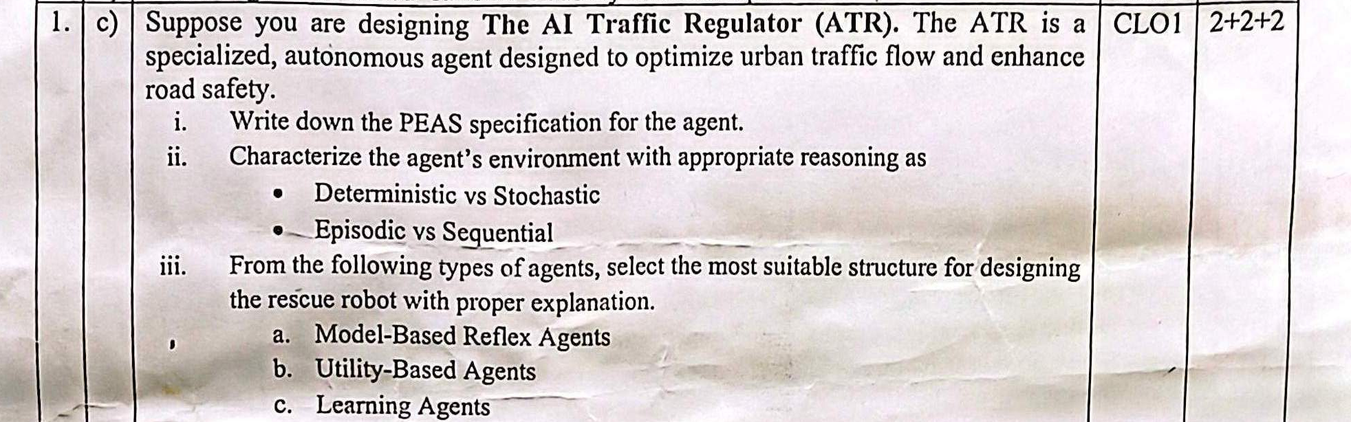
i. PEAS Specification for AI Traffic Regulator (ATR):
| Component | Detailed Description |
|---|---|
| Performance Measure (P) | Maximize vehicle throughput, minimize intersection wait time / queue delay, zero traffic accidents/fatalities, prioritize emergency vehicles (ambulances/fire engines), minimize vehicle emissions. |
| Environment (E) | Multi-lane urban road network, signalized intersections, diverse vehicles (cars, buses, bikes), pedestrian crosswalks, unpredictable weather, roadwork disruptions. |
| Actuators (A) | Variable traffic light phase timers, digital variable message signs (VMS), automated lane control signals, connected vehicle speed advisory broadcasts. |
| Sensors (S) | High-resolution CCTV traffic cameras, underground inductive loop sensors, LiDAR traffic scanners, radar speed guns, emergency vehicle transponder transceivers. |
ii. Environment Characterization with Reasoning:
- Deterministic vs. Stochastic → Stochastic: Traffic flow cannot be calculated deterministically. Driver reaction times, vehicle breakdowns, sudden lane changes, and pedestrian crossings introduce fundamental randomness.
- Episodic vs. Sequential → Sequential: A traffic signal decision made at 8:00 AM directly impacts traffic queue density and bottleneck formation at 8:15 AM. Every action cascades into future states.
iii. Agent Architecture Selection:
Most Suitable Structure: Utility-Based Agent (with Learning):
Reasoning: A Simple Reflex agent cannot handle partial observability and creates phantom gridlocks. A Goal-Based agent only recognizes binary goals ("clear the junction: Yes/No"), but cannot balance trade-offs. Traffic control inherently involves conflicting objectives (e.g., delaying side-street vehicles by 30 seconds to allow a massive 100-car highway platoon to pass, or pausing all traffic for an ambulance). A Utility-Based Agent maps state sequences to continuous real-valued happiness scores, enabling optimal mathematical trade-offs under heavy uncertainty.
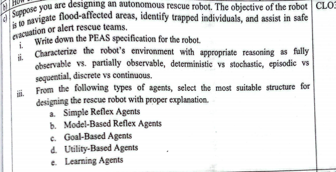
i. PEAS Specification for Autonomous Rescue Robot:
| Component | Technical Specification |
|---|---|
| Performance Measure (P) | Number of human victims identified and rescued, search completion time, robot survival/damage minimization, battery energy efficiency, zero false distress alerts. |
| Environment (E) | Flood-inundated geographical zones, submerged obstacles, fast-flowing water currents, collapsed buildings, rain/storm weather, trapped victims. |
| Actuators (A) | Motorized water thrusters/crawler tracks, robotic extraction arm, inflatable rescue raft deployment mechanism, emergency siren/strobe beacon, satellite radio transmitter. |
| Sensors (S) | Forward-looking infrared (FLIR) thermal cameras (detecting body heat), underwater sonar, optical cameras, GPS receiver, water level/depth sensors, IMU gyroscope. |
ii. Characterization of Environment (with Reasoning):
- Fully vs. Partially Observable → Partially Observable: Murky floodwaters, collapsed roofs, and rain obscure human victims and submerged hazards from sensor range.
- Deterministic vs. Stochastic → Stochastic: Shifting flood currents, drifting debris, and changing weather cannot be predicted with 100% certainty.
- Episodic vs. Sequential → Sequential: Navigating through a narrow waterway consumes battery and alters the robot's future reachability to distant victims.
- Discrete vs. Continuous → Continuous: Robot position, velocity, water currents, steering angles, and sensor readings vary continuously over real numbers.
iii. Agent Architecture Selection:
Most Suitable Structure: Utility-Based Agent (with Learning):
Reasoning: In life-threatening rescue missions, goals frequently conflict under severe resource constraints (e.g., whether to rescue one critically injured person immediately versus searching for a group of five victims before the robot's battery depletes). Only a Utility-Based Agent can assign real-valued utilities to risky alternatives, calculating expected utility to make rational trade-offs between speed, victim survival probability, and robot risk.
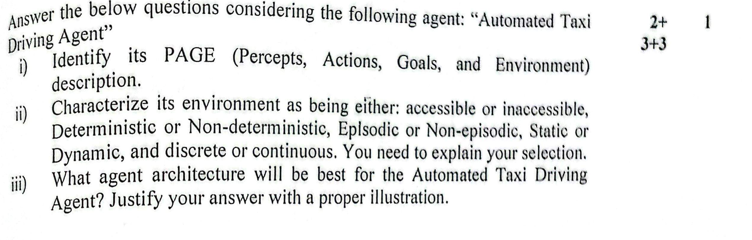
i. PAGE / PEAS Description for Automated Taxi Driver:
- Percepts (Sensors): Video feed from 360° cameras, LiDAR 3D point clouds, radar echoes, GPS coordinates, speedometer data, engine diagnostics, passenger voice commands.
- Actions (Actuators): Steering wheel angle, electronic throttle acceleration, brake pressure, gear shift, turn signals, horn, passenger cabin UI.
- Goals: Deliver passengers safely, legally, comfortably, and promptly to destination while maximizing operating profit.
- Environment: City streets, expressways, dynamic traffic, erratic pedestrians, road detours, weather conditions.
ii. Characterization of the Environment:
- Inaccessible (Partially Observable): The taxi cannot perceive what is around blind corners or inside the minds of other human drivers.
- Non-deterministic (Stochastic): Tires can skid, pedestrians can step off curbs without looking, and other vehicles behave unpredictably.
- Non-episodic (Sequential): Every driving action (e.g. changing lanes) fundamentally affects future opportunities, positioning, and safety.
- Dynamic: Traffic and pedestrians keep moving while the agent's computer processes sensor data and deliberates.
- Continuous: Velocity, steering angle, time, and coordinates are all continuous variables.
iii. Best Architecture & Justification:
Model-Based Utility Agent with Learning: Must maintain an internal model of the world (road network map, tracking obscured vehicles) and calculate continuous trade-offs between safety, ride smoothness, and travel speed using expected utility theory.

i. PEAS Specification for Game Playing AI - Chess:
- P (Performance): Win (+1), Draw (0), Loss (-1); board material evaluation, center control, king safety.
- E (Environment): 64-square chessboard, 32 game pieces, opposing human or AI player.
- A (Actuators): Display generated move on screen (algebraic notation like
e2-e4) or robotic manipulator arm. - S (Sensors): Digital board state input / optical camera tracking piece coordinates.
ii. Characterization of the Environment:
- Fully Observable: The complete state of the board and all pieces are visible at all times.
- Deterministic: Each move has a 100% predictable transition with zero random chance.
- Static: The board state does not change while the agent is calculating its next move (apart from the chess clock).
- Discrete: A finite set of discrete board squares and legal move actions.
- Multi-Agent (Competitive / Zero-Sum): Two agents competing where one agent's gain is exactly the opponent's loss.
| Architecture | How it Decides | Key Internal Components | Critical Limitation / Strength |
|---|---|---|---|
| 1. Simple Reflex | Condition-Action rules: IF condition THEN action |
Sensors \(\to\) Condition-Action Rules \(\to\) Actuators | No memory. Trapped in infinite loops in partially observable worlds. |
| 2. Model-Based | Maintains internal state reflecting unobserved world | Transition models: how world moves + what my actions do | Tracks history, but lacks explicit goal-directed search. |
| 3. Goal-Based | Combines state with goal descriptions using search/planning | Internal state + Goal specification + Planning search | Can find paths to targets, but cannot balance competing trade-offs. |
| 4. Utility-Based | Maps state to a real-valued utility score \(U(s)\) | Utility function: balances trade-offs (speed, safety, cost) | Optimal decision-making under multi-objective uncertainty. |
| 5. Learning Agent | Improves behavior over time from environmental feedback | Critic, Learning Element, Performance Element, Problem Generator | Adapts to novel, unmodeled environments. Problem generator ensures exploration. |
Which architecture is best for an Autonomous Rescue Robot or Automated Taxi?
Answer: Utility-Based Agent with a Learning Element.
Justification: A rescue robot operates under severe life-or-death trade-offs (e.g. risking battery life vs. rescuing an extra victim). A binary goal is insufficient; it must maximize a utility function: \(U = w_1(\text{Victims Saved}) - w_2(\text{Risk to Robot}) - w_3(\text{Time})\). The learning element adapts traction and path planning to previously unmodeled disaster terrain.
Basic Functioning: Acts based exclusively on the current percept, completely ignoring all historical percept sequences.
Condition-Action Rule: Operates using IF [Condition] THEN [Action] associations. Example: "If someone is detected in front of the car, initiate-braking."
Slide Examples (Slide 54):
- Touching a Hot Pan: Human spinal reflex immediately pulls the hand away from the burning surface without waiting for cerebral deliberation.
- Automobile Airbag Deployment: Accelerometer detects a deceleration impulse exceeding safety threshold \(\to\) triggers pyrotechnic inflator immediately.
Fatal Limitation: Fails catastrophically under partial observability (e.g., if a preceding car has broken brake lights, the reflex agent cannot deduce that the vehicle is stopped). Prone to infinite action loops.
Handling Partial Observability: Specifically engineered to operate in partially observable environments by maintaining an Internal State that reflects unobserved aspects of the world.
Updating the Internal State: Combines percept history with two core forms of domain knowledge: (1) How the world evolves independently of the agent, and (2) How the agent's own actions affect the world.
Slide Example: Autonomous Driving Vehicle (Slide 57):
- Internal Model: Contains digital road maps, traffic regulations, lane topologies, and typical traffic flows.
- Sensors: Cameras and sensors perceive traffic signals, road signs, surrounding vehicles, pedestrians, and pavement condition.
- Updating Knowledge: Continuously updates its model in real-time as it drives—registering newly opened construction zones, sudden traffic jams, or detours.
- Decision Making: Stops when approaching red light; proceeds when light turns green and intersection is clear.
- Learning Over Time: Refines its predictive model to estimate accurate journey times taking dynamic traffic patterns into account.
Goal Information: An extension of model-based reflex agents that incorporates explicit Goal descriptions specifying desirable terminal states. Instead of reacting reflexively, the agent considers sequences of actions (planning and search) to achieve the goal.
Slide Example 1: Rain & Braking Adaptation (Slide 59): If it begins to rain, a goal-based vehicle agent updates its model regarding reduced tire friction and braking distances, dynamically increasing following distances to reach its destination safely.
Slide Example 2: Automated Vacuum Cleaner (Slide 60):
- Goal: Clean the entire floor area.
- Perception: Senses current room coordinate and whether the current tile is clean or dirty.
- Actions:
Move(changes position across floor grid) andClean(activates suction on dirty tiles). - Decision-Making: Cleans dirty spots; moves toward unvisited dirty rooms if current room is clean.
- Goal Achievement: Halts operation once all tiles detect zero dirt, indicating the floor is clean!
Utility Metric: Goals provide only a binary distinction between winning and losing. Utility-based agents use an internalized Utility Function (\(U: S \to \mathbb{R}\)) that quantifies "how happy or satisfied" the agent is with a particular world state.
Handling Trade-offs (Slide 61): Multiple routes reach a destination, but some are faster, safer, or cheaper. A utility function balances these competing objectives to choose the optimal compromise.
Slide Example: Smart Thermostat (Slide 62):
- Goal: Maintain a comfortable indoor home temperature.
- Perception: Measures ambient temperature and learns occupant schedule preferences.
- Actions:
Heat,Cool, orIdle / Maintain. - Utility Calculation: Balances occupant thermal comfort against electricity consumption costs.
- Decision-Making: Chooses heating/cooling intervals to maximize net utility—lowering heating slightly during peak tariff hours when occupants are asleep.
| Feature (Slide 63) | Simple Reflex Agents | Model-Based Reflex Agents | Goal-Based Agents | Utility-Based Agents |
|---|---|---|---|---|
| Basis of Operation | Operate on the current percept only. | Use an internal model to keep track of the world state. | Act to achieve defined goals. | Act to maximize a utility function. |
| Environment Interaction | React to stimuli with conditioned actions. | Update internal state from current state and action history. | Consider future consequences of actions. | Evaluate success based on a utility function. |
| Flexibility | Very limited; cannot handle new situations well. | More flexible; can handle unseen scenarios to an extent. | Flexible; can adapt actions to achieve goals in changing environments. | Highly flexible; aims for optimal performance under trade-offs. |
| Learning Ability | None; they do not learn from past actions. | Limited; can improve the internal model with new experiences. | Can learn better strategies to achieve goals. | Can adjust utility function based on outcomes. |
| Concrete Slide Example | Thermostat controlling a heating system; car with anti-lock brakes. | Autonomous vehicle updating its internal road map and traffic detours. | Chess-playing AI; automated vacuum cleaner robot. | Investment portfolio AI maximizing return while minimizing financial risk. |
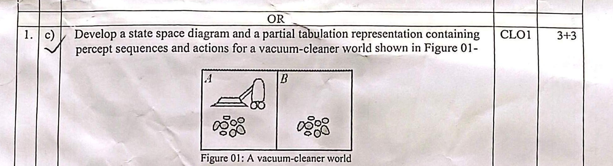
1. State Space Diagram for Vacuum-Cleaner World:
The vacuum world in Figure 01 has 2 locations (\(A\) and \(B\)), and each location can be either Clean (\(C\)) or Dirty (\(D\)).
Total discrete states = \(2 \text{ (Agent locations)} \times 2^2 \text{ (Clean/Dirty combinations)} = 8 \text{ States}\):
  State 1: [Agent in A, A: Dirty, B: Dirty]   State 2: [Agent in B, A: Dirty, B: Dirty]
  State 3: [Agent in A, A: Clean, B: Dirty]   State 4: [Agent in B, A: Clean, B: Dirty]
  State 5: [Agent in A, A: Dirty, B: Clean]   State 6: [Agent in B, A: Dirty, B: Clean]
  State 7: [Agent in A, A: Clean, B: Clean]   State 8: [Agent in B, A: Clean, B: Clean]
Actions: Left, Right, Suck. From State 1, Suck → State 3; Right → State 2. From State 2, Suck → State 6; Left → State 1. All 8 states form a complete directed graph with transitions governed by the movement and cleaning actions.
2. Partial Tabulation Representation (Percept Sequences → Action):
| Percept Sequence | Action | Explanation |
|---|---|---|
| \([(\text{A}, \text{Clean})]\) | Right | Current square is clean; navigate to adjacent room. |
| \([(\text{A}, \text{Dirty})]\) | Suck | Dirt detected in current square; clean immediately. |
| \([(\text{B}, \text{Clean})]\) | Left | Current square is clean; return to inspect room A. |
| \([(\text{B}, \text{Dirty})]\) | Suck | Clean dirt in room B. |
| \([(\text{A}, \text{Dirty}), (\text{A}, \text{Clean})]\) | Right | Room A was cleaned; proceed to Room B. |
| \([(\text{A}, \text{Clean}), (\text{B}, \text{Dirty})]\) | Suck | Arrived in Room B and found dirt; clean it. |
| \([(\text{A}, \text{Clean}), (\text{B}, \text{Clean})]\) | NoOp | Both rooms verified clean; idle to conserve energy. |
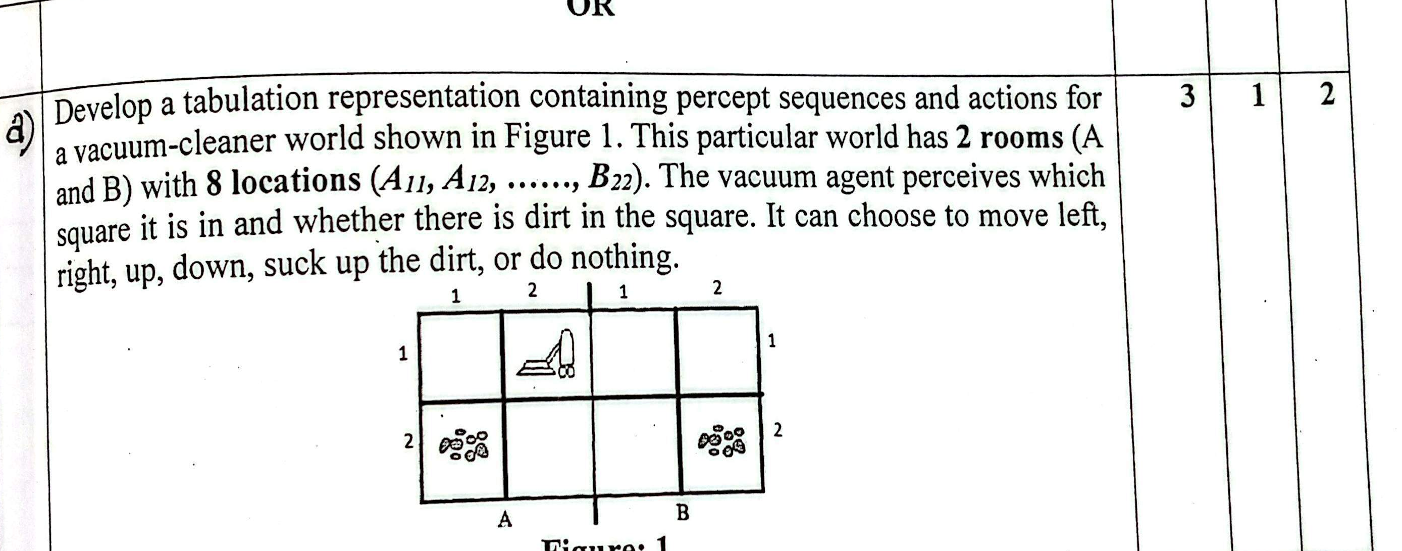
Vacuum Cleaner World with 2 Rooms and 8 Locations (\(A_{11}, A_{12}, A_{21}, A_{22}, B_{11}, B_{12}, B_{21}, B_{22}\)):
Actions Available: Left, Right, Up, Down, Suck, NoOp.
| Current Location | Status | Recommended Action | Next State Target |
|---|---|---|---|
| \(A_{11}\) | Dirty | Suck | \(A_{11}\) Clean |
| \(A_{11}\) | Clean | Right | Inspect \(A_{12}\) |
| \(A_{12}\) | Clean | Down | Inspect \(A_{22}\) |
| \(A_{22}\) | Clean | Left | Inspect \(A_{21}\) |
| \(A_{21}\) | Clean | Right → Cross Room | Move into Room B (\(B_{21}\)) |
| \(B_{21}\) | Dirty | Suck | \(B_{21}\) Clean |
| \(B_{22}\) | Clean (all clean) | NoOp | Conserve power |
A classical search problem is formally formulated by 5 components:
- Initial State: The starting state of the agent (e.g. \(\text{In}(Arad)\)).
- Actions: The set of valid actions at state \(s\): \(A(s)\).
- Transition Model: The result of executing action \(a\) in state \(s\): \(\text{Result}(s, a) = s'\).
- Goal Test: Predicate checking if state is a goal: \(\text{GoalTest}(s) \in \{\text{True}, \text{False}\}\).
- Path Cost: Numeric cost of the path, sum of step costs: \(c(s, a, s')\).
In a 2-room vacuum world (Rooms A & B):
Total States = 2 (agent locations) × 2² (dirt status of rooms) = 2 × 4 = 8 distinct states.

                     STATE 1: (A, D, D)  ──── Right ────>  STATE 2: (B, D, D)
                          │                                      │
                         Suck                                   Suck
                          ▼                                      ▼
                     STATE 3: (A, C, D)  ──── Right ────>  STATE 4: (B, C, D)
                          │                                      │
                        Right                                   Suck
                          ▼                                      ▼
                     STATE 5: (A, D, C)  <─── Left  ─────  STATE 6: (B, D, C)
                          │                                      │
                         Suck                                   Left
                          ▼                                      ▼
                 ┌──> STATE 7: (A, C, C)  ──── Right ────>  STATE 8: (B, C, C) <──┐
                 │        │                                      │                │
                 │      [Goal]                                 [Goal]             │
                 └─────── Left ──────────────────────────────────┘────────────────┘
8-Location Variant (Autumn 2023): With 8 sub-locations, total states = \(8 \times 2^8 = 8 \times 256 = \mathbf{2,048 \text{ states}}\). This proves why state abstraction is necessary to prevent state space explosion!
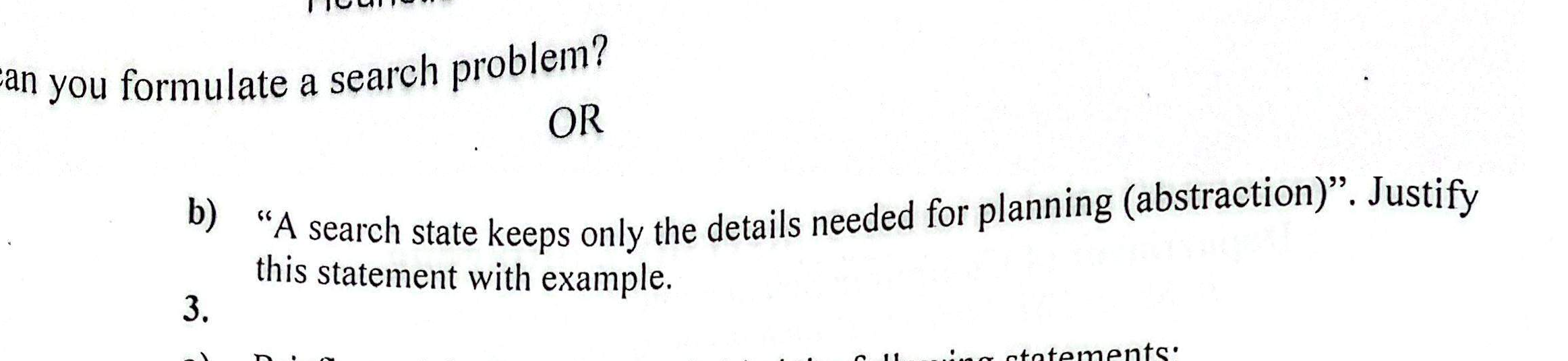
1. How to Formulate a Search Problem (The 5 Core Elements):
- Initial State \(s_0\): The state in which the agent starts (e.g. \(\text{In}(Arad)\)).
- Actions \(ACTIONS(s)\): The set of legal moves executable from state \(s\).
- Transition Model \(RESULT(s, a)\): Formal description of what each action does, returning successor state \(s'\).
- Goal Test \(GOAL\text{-}TEST(s)\): A boolean predicate checking whether state \(s\) satisfies the goal condition (e.g. \(s == \text{In}(Bucharest)\)).
- Path Cost Function \(c(s, a, s')\) & Total Cost \(g(n)\): Sum of individual step costs measuring the quality of the path.
2. Justification: "A search state keeps only the details needed for planning (abstraction)":
In real life, a traveling agent has infinite physical parameters: exact tire pressure, paint color, radio frequency, passenger clothing, and wind speed. If all these details were included in the state representation, the state space would become infinite and computationally intractable.
Abstraction is the deliberate process of removing irrelevant real-world details, preserving only the features essential for problem solving. In route planning, the state needs only the current city node (e.g., \(\text{In}(Sibiu)\)). All other features are abstracted away.
3. Explicit vs. Implicit State Space Representations (Spring 2022 Q2.b):
- Explicit Data Structure: Every state and transition edge is explicitly pre-allocated in memory (e.g., Adjacency Matrix, Adjacency List). Only usable for small graphs (\(|V| \le 10^5\)).
- Implicit Data Structure: States are generated dynamically on demand using generative successor functions / rules (e.g., in Chess or 8-Puzzle with \(10^{40}\) states, the graph is generated dynamically during search tree expansion).
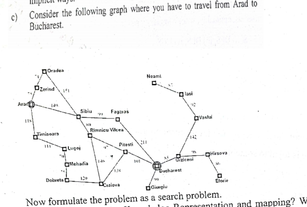
Formal Search Problem Formulation: Traveling from Arad to Bucharest:
- Initial State: \(\text{In}(Arad)\)
- Actions Available: \(\{ \text{Go}(c) \mid c \text{ is directly connected to current city by road} \}\)
- Transition Model: \(RESULT(\text{In}(x), \text{Go}(y)) = \text{In}(y)\) if road \((x, y)\) exists.
- Goal Test: \(State == \text{In}(Bucharest)\)
- Path Cost: Sum of road segment distances in kilometers: \(g(n) = \sum \text{distance}(x, y)\).
Searching Techniques & Heuristic Problem Solving
In uninformed (blind) search, the agent has no estimate \(h(n)\) of how far a state is from the goal. It only knows step costs and valid actions. How do we systematically explore paths without wandering aimlessly?
- BFS (Breadth-First): Explores shallowest nodes first using a FIFO Queue. Spreads outward in concentric ripples.
- DFS (Depth-First): Explores deepest nodes first using a LIFO Stack. Wanders down a corridor until hitting a dead end.
- DLS (Depth-Limited): DFS bounded by an artificial depth limit \(l\) to prevent falling into infinite paths.
- UCS (Uniform-Cost): Explores the cheapest path so far using a Priority Queue ordered by \(g(n)\).
| Algorithm | Data Structure | Completeness | Optimality | Time Complexity | Space Complexity | Primary Bottleneck |
|---|---|---|---|---|---|---|
| BFS | FIFO Queue | Yes (if \(b\) finite) | Yes (if step costs equal) | \(O(b^d)\) | \(O(b^d)\) (Exponential) | Memory exhaustion (stores entire frontier) |
| DFS | LIFO Stack | No (loops in infinite trees) | No | \(O(b^m)\) | \(O(b \cdot m)\) (Linear) | Can get trapped down infinite branches |
| DLS | LIFO Stack (depth \(\le l\)) | No (if \(d > l\)) | No (if \(l > d\)) | \(O(b^l)\) | \(O(b \cdot l)\) (Linear) | Incomplete if limit \(l\) is chosen too small |
| UCS | Priority Queue (\(g(n)\)) | Yes (if \(c \ge \epsilon > 0\)) | Yes (arbitrary costs) | \(O(b^{1 + \lfloor C^* / \epsilon floor})\) | \(O(b^{1 + \lfloor C^* / \epsilon floor})\) | Explores every direction of low cost |
Breadth-First Search explores all neighboring nodes at the current depth level before proceeding to the next level. It is implemented using a First-In First-Out (FIFO) queue: new nodes (deeper) are enqueued at the back, and shallowest nodes are dequeued from the front first.
Graph Topology: Vertices \(\{A, B, C, D, E, F, G\}\). Edges connect: \(A-B, A-D, A-E, B-E, C-E, C-F, C-G, D-E, E-F, F-G\). Starting vertex = A.
| Step | Operation Performed | Visited Adjacent Vertices | FIFO Queue State |
|---|---|---|---|
| Step 1 | Select starting vertex A (visit A) and insert into Queue. | A | [ A ] |
| Step 2 | Delete A from Queue. Visit all unvisited adjacent vertices of A: D, E, B. Enqueue them. | D, E, B | [ D, E, B ] |
| Step 3 | Delete D from Queue. Visit unvisited adjacent of D (none). | — | [ E, B ] |
| Step 4 | Delete E from Queue. Visit unvisited adjacent of E: C, F. Enqueue them. | C, F | [ B, C, F ] |
| Step 5 | Delete B from Queue. Visit unvisited adjacent of B (none). | — | [ C, F ] |
| Step 6 | Delete C from Queue. Visit unvisited adjacent of C: G. Enqueue G. | G | [ F, G ] |
| Step 7 | Delete F from Queue. Visit unvisited adjacent of F (none). | — | [ G ] |
| Step 8 | Delete G from Queue. Visit unvisited adjacent of G (none). Queue is now Empty! | — | [ ] (Empty) |
Resulting BFS Spanning Tree (Slide 75): Formed by edges \((A-D), (A-E), (A-B), (E-C), (E-F), (C-G)\). Level 0: A; Level 1: D, E, B; Level 2: C, F; Level 3: G.
Graph Topology: Vertices \(\{A, B, C, D, E\}\). Edges: \(A-B, A-C, B-D, B-E, C-D, D-E\). Starting vertex = A.
- Step 1: Select start vertex A, insert into Queue \(\to\) Queue =
[ A ]. - Step 2: Delete A from Queue. Visit unvisited neighbors of A: B, C. Enqueue them \(\to\) Queue =
[ B, C ]. - Step 3: Delete B from Queue. Visit unvisited neighbors of B: D, E. Enqueue them \(\to\) Queue =
[ C, D, E ]. - Step 4: Delete C from Queue. Visit unvisited neighbors of C (D is already visited) \(\to\) Queue =
[ D, E ]. - Step 5: Delete D from Queue. No unvisited neighbors \(\to\) Queue =
[ E ]. - Step 6: Delete E from Queue. No unvisited neighbors \(\to\) Queue =
[ ]. - Step 7: Queue is empty! BFS terminates. Resulting Spanning Tree edges: \((A-B), (A-C), (B-D), (B-E)\).
Depth-First Search explores as far as possible along each branch before backtracking. It traverses the depth of a tree or graph using a Last-In First-Out (LIFO) stack or recursive function calls.
Graph vertices \(\{A, B, C, D, E, F, G\}\). Starting vertex = A. Following alphabetical / adjacency order:
| Step | Operation & Action | LIFO Stack State (Bottom \(\to\) Top) | Action Type |
|---|---|---|---|
| Step 1 | Select vertex A (visit A). Push A to stack. | [ A ] (top=A) | Forward Push |
| Step 2 | Visit unvisited adjacent of A: B. Push B. | [ A, B ] (top=B) | Forward Push |
| Step 3 | Visit unvisited adjacent of B: C. Push C. | [ A, B, C ] (top=C) | Forward Push |
| Step 4 | Visit unvisited adjacent of C: E. Push E. | [ A, B, C, E ] (top=E) | Forward Push |
| Step 5 | Visit unvisited adjacent of E: D. Push D. | [ A, B, C, E, D ] (top=D) | Forward Push |
| Step 6 | No unvisited vertices from D. Backtrack! Pop D. | [ A, B, C, E ] (top=E) | Backtrack Pop |
| Step 7 | From E, visit unvisited adjacent: F. Push F. | [ A, B, C, E, F ] (top=F) | Forward Push |
| Step 8 | From F, visit unvisited adjacent: G. Push G. | [ A, B, C, E, F, G ] (top=G) | Forward Push |
| Step 9 | No unvisited vertices from G. Backtrack! Pop G. | [ A, B, C, E, F ] (top=F) | Backtrack Pop |
| Step 10 | No unvisited vertices from F. Backtrack! Pop F. | [ A, B, C, E ] (top=E) | Backtrack Pop |
| Step 11 | No unvisited vertices from E. Backtrack! Pop E. | [ A, B, C ] (top=C) | Backtrack Pop |
| Step 12 | No unvisited vertices from C. Backtrack! Pop C. | [ A, B ] (top=B) | Backtrack Pop |
| Step 13 | No unvisited vertices from B. Backtrack! Pop B. | [ A ] (top=A) | Backtrack Pop |
| Step 14 | No unvisited vertices from A. Backtrack! Pop A. Stack is Empty! Terminate. | [ ] (Empty) | Complete |
Resulting DFS Spanning Tree (Slide 88): Directed spine: \(A \to B \to C \to E \to D\), and branching from E to \(F \to G\).
Graph vertices \(\{A, B, C, D, E\}\). Starting at A:
- Push A \(\to\) Stack:
[A]. - Visit adjacent B \(\to\) Push B \(\to\) Stack:
[A, B]. - Visit adjacent D \(\to\) Push D \(\to\) Stack:
[A, B, D]. - Visit adjacent C \(\to\) Push C \(\to\) Stack:
[A, B, D, C]. - No unvisited from C \(\to\) Pop C \(\to\) Stack:
[A, B, D]. - From D, visit unvisited E \(\to\) Push E \(\to\) Stack:
[A, B, D, E]. - No unvisited from E \(\to\) Pop E \(\to\) Stack:
[A, B, D]. - No unvisited from D \(\to\) Pop D \(\to\) Stack:
[A, B]. - No unvisited from B \(\to\) Pop B \(\to\) Stack:
[A]. - No unvisited from A \(\to\) Pop A \(\to\) Stack:
[]. Terminate!
Uniform Cost Search (UCS) is an extension of Breadth-First Search that takes into account the cumulative path cost \(g(n)\) of reaching each node to find the lowest-cost path to the goal.
                                     ( a )
                                    /     \
                                 1 /       \ 5
                                  /         \
                                ( b )       ( c )
                                /   \       / | \
                             2 /   6 \   1 /  |3 \ 4
                              /       \   /   |   \
                            ( d )    ( e)( f )( g )( h )
Starting at root \(a\) with \(g(a) = 0\):
- From \(a\): Children are \(b\) (cost 1) and \(c\) (cost 5). Priority queue: \(\{b: 1, c: 5\}\).
- Dequeue lowest cost node: \(b\) (cost 1). Expand \(b\) \(\to\) \(d\) (cost \(1+2=3\)) and \(e\) (cost \(1+6=7\)). Queue: \(\{d: 3, c: 5, e: 7\}\).
- Dequeue lowest: \(d\) (cost 3).
- Dequeue lowest: \(c\) (cost 5). Expand \(c\) \(\to\) \(f\) (cost \(5+1=6\)), \(g\) (cost \(5+3=8\)), \(h\) (cost \(5+4=9\)). Queue: \(\{f: 6, e: 7, g: 8, h: 9\}\).
- Dequeue lowest: \(f\) (cost 6).
- Dequeue lowest: \(e\) (cost 7).
- Dequeue lowest: \(g\) (cost 8).
- Dequeue lowest: \(h\) (cost 9).
Final Expansion Sequence: $$\mathbf{a \;\longrightarrow\; b \;\longrightarrow\; d \;\longrightarrow\; c \;\longrightarrow\; f \;\longrightarrow\; e \;\longrightarrow\; g \;\longrightarrow\; h}$$

Differentiate BFS, DFS, DLS, and UCS:
| Algorithm | Completeness | Optimality | Time Complexity | Space Complexity |
|---|---|---|---|---|
| BFS (Breadth-First) | Yes (if branching factor \(b\) is finite) | Yes (if step cost is uniform / constant) | \(O(b^d)\) | \(O(b^d)\) (Exponential - major bottleneck) |
| DFS (Depth-First) | No (fails in infinite paths/cycles; Yes in finite spaces) | No (can return deep non-optimal paths) | \(O(b^m)\) | \(O(b \cdot m)\) (Linear - highly memory efficient) |
| DLS (Depth-Limited) | No (incomplete if goal depth \(d >\) limit \(l\)) | No (returns first solution found within limit) | \(O(b^l)\) | \(O(b \cdot l)\) (Linear) |
| UCS (Uniform-Cost) | Yes (if step costs \(\ge \epsilon > 0\)) | Yes (always finds lowest-cost path) | \(O(b^{1 + \lfloor C^* / \epsilon floor})\) | \(O(b^{1 + \lfloor C^* / \epsilon floor})\) |
Where \(b\) = branching factor, \(d\) = shallowest goal depth, \(m\) = maximum tree depth, \(l\) = depth limit, \(C^*\) = optimal path cost, \(\epsilon\) = minimum step cost.
Bidirectional Search is an uninformed search strategy that simultaneously executes two separate searches:
- A forward search starting from the initial state \(S\).
- A backward search running inversely from the goal state \(G\).
The two searches advance through the state space toward one another and terminate when their search frontiers intersect (i.e., a common node is generated in both directions). Replacing the global goal test with a frontier intersection check detects the solution path in half the search depth.
Suppose a problem has branching factor \(b = 10\) and the goal is at depth \(d = 8\):
- Standard Unidirectional BFS: Explores \(b^d = 10^8 = 100,000,000\) nodes.
- Bidirectional Search: Each direction explores to depth \(d/2 = 4\). The total nodes generated is \(b^{d/2} + b^{d/2} = 10^4 + 10^4 = 20,000\) nodes!
This achieves an astronomical \(5,000\times\) reduction in search operations!
          FORWARD FRONTIER                       BACKWARD FRONTIER
             FROM START                             FROM GOAL
               (S)                                    (G)
              /   \                                  /   \
             o     o                                o     o
            / \   / \                              / \   / \
           o   o o   o                            o   o o   o
          └─────┬─────┘                          └─────┬─────┘
                │                                      │
                ▼                                      ▼
           [FRONTIER 1] ◄════════ INTERSECT ════════► [FRONTIER 2]
                                (Meeting Node)
| Evaluation Parameter | Bidirectional Search Performance | Formal Justification (Slides 100–101) |
|---|---|---|
| Completeness | Complete | Guaranteed to find a solution if the search space is finite and step costs are positive. |
| Optimality | Optimal | Optimal if both directions use Breadth-First Search (uniform step costs) or Uniform Cost Search. |
| Time Complexity | \(O(b^{d/2})\) | Each search only explores to depth \(d/2\), dramatically shrinking the tree exponent. |
| Space Complexity | \(O(b^{d/2})\) | Major Disadvantage: At least one of the two search frontiers (and its visited closed list) must remain fully buffered in memory to test for intersections. |
| Implementation Overhead | High | Requires calculating predecessor states (difficult in irreversible games), synchronizing two queues, and constant hash checks for frontier intersections. |
The definitive comparative synthesis of all uninformed search algorithms from Figure 3.21 of the course curriculum:
| Criterion | Breadth-First (BFS) | Uniform-Cost (UCS) | Depth-First (DFS) | Depth-Limited (DLS) | Iterative Deepening (IDS) | Bidirectional (BDS) |
|---|---|---|---|---|---|---|
| Complete? | Yesa | Yesa,b | No | No | Yesa | Yesa,d |
| Time Complexity | \(O(b^d)\) | \(O(b^{1 + \lfloor C^* / \epsilon \rfloor})\) | \(O(b^m)\) | \(O(b^\ell)\) | \(O(b^d)\) | \(O(b^{d/2})\) |
| Space Complexity | \(O(b^d)\) | \(O(b^{1 + \lfloor C^* / \epsilon \rfloor})\) | \(O(b \cdot m)\) | \(O(b \cdot \ell)\) | \(O(b \cdot d)\) | \(O(b^{d/2})\) |
| Optimal? | Yesc | Yes | No | No | Yesc | Yesc,d |
Notation: \(b\) = branching factor; \(d\) = depth of shallowest solution; \(m\) = maximum depth of search tree; \(\ell\) = depth limit; \(C^*\) = optimal path cost; \(\epsilon\) = minimum edge cost bound.
Footnote caveats: a Complete if \(b\) is finite. b Complete if step costs \(\ge \epsilon > 0\). c Optimal if step costs are all identical. d If both directions use breadth-first search.
- Blind Exploration: Uninformed strategies lack domain-specific heuristics. They examine nodes blindly based solely on structural topology, generating millions of unpromising states.
- Inefficiency in Complex Spaces: In large search spaces (e.g. 15-puzzle, TSP, routing), combinatorial explosion renders \(O(b^d)\) memory and time completely intractable without domain guidance.
A heuristic function \(h(n)\) is an educated estimate of the cheapest cost from state \(n\) to a goal state.
- Admissibility: \(0 \le h(n) \le h^*(n)\) for all \(n\). It never overestimates true remaining cost. Guarantees optimality for \(A^*\) Tree Search.
- Consistency (Monotonicity): \(h(n) \le c(n, a, n') + h(n')\) (Triangle Inequality). Guarantees optimality for \(A^*\) Graph Search without reopening closed nodes.
- Dominance: If \(h_2(n) \ge h_1(n)\) for all \(n\) and both are admissible, \(h_2\) dominates \(h_1\) and expands fewer or equal nodes.
    CURRENT STATE                    GOAL STATE
    ┌───┬───┬───┐                   ┌───┬───┬───┐
    │ 1 │ 2 │ 3 │                   │ 1 │ 2 │ 3 │
    ├───┼───┼───┤                   ├───┼───┼───┤
    │ - │ 4 │ 6 │                   │ 4 │ 5 │ 6 │
    ├───┼───┼───┤                   ├───┼───┼───┤
    │ 7 │ 5 │ 8 │                   │ 7 │ 8 │ - │
    └───┴───┴───┘                   └───┴───┴───┘
- Misplaced Tiles (\(h_1\)): Counts tiles out of position. Tiles 4, 5, 8 are misplaced \(\implies \mathbf{h_1 = 3}\).
- Manhattan Distance (\(h_2\)): Sum of grid displacements: \(h_2 = |2-2|+|2-1| \text{ (tile 4)} + |3-2|+|2-2| \text{ (tile 5)} + |3-3|+|3-2| \text{ (tile 8)} = 1 + 1 + 1 = \mathbf{3}\).

1. Definition of Heuristic:
A Heuristic is a problem-solving rule of thumb or domain-specific evaluation function \(h(n)\) that estimates the remaining cost from current node \(n\) to the nearest goal state. It does not guarantee a perfect solution by itself, but dramatically prunes the search space by guiding the algorithm toward promising paths.
2. Heuristics of the 8-Queens Problem:
- Cost Heuristic \(h(n)\): The number of pairs of queens that are attacking each other (either directly or indirectly along the same row or diagonal). A goal state has \(h(n) = 0\).
- Fitness Heuristic \(f(n)\): The number of non-attacking pairs of queens: \(f(n) = \binom{8}{2} - h(n) = 28 - h(n)\). The goal state maximizes fitness to \(f(n) = 28\).
3. Heuristics of the 8-Puzzle Problem (Autumn 2023 Q1.b):
- \(h_1\) (Misplaced Tiles): The number of tiles that are not in their target goal positions. It is admissible because every misplaced tile must be moved at least once.
- \(h_2\) (Manhattan Distance): The sum of vertical and horizontal distances that tiles are displaced from their goal positions: \(\sum |x_i - x_{goal}| + |y_i - y_{goal}|\). \(h_2\) strictly dominates \(h_1\) (\(h_2(n) \ge h_1(n)\) for all \(n\)) and is both admissible and consistent.
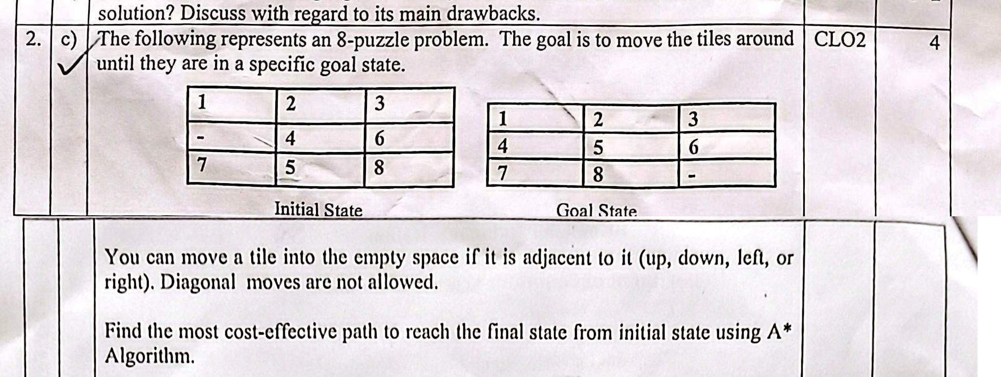
8-Puzzle Problem Solution Using A* Algorithm:
Initial State:
[ 1  2  3 ]
[ -  4  6 ]   (Blank '-' is at row 2, col 1)
[ 7  5  8 ]
Goal State:
[ 1  2  3 ]
[ 4  5  6 ]
[ 7  8  - ]   (Blank '-' is at row 3, col 3)
Heuristic Function \(h(n)\): Manhattan Distance (Sum of distances of each tile from its target coordinates):
- Initial State \(S_0\): Tiles 1, 2, 3, 7 are already in position. Tile 4 is at (2,2), target is (2,1) → dist = 1. Tile 5 is at (3,2), target is (2,2) → dist = 1. Tile 6 is at (2,3), target is (2,3) → dist = 0. Tile 8 is at (3,3), target is (3,2) → dist = 1. Total \(h(S_0) = 1 + 1 + 0 + 1 = 3\).
- \(g(S_0) = 0 \implies f(S_0) = g + h = 0 + 3 = 3\).
Step-by-Step Search Tree Expansion:
- Step 1: Expand \(S_0\). Legal moves for Blank from (2,1):
- Move UP: Blank swaps with 1 → \(g=1, h=4, f=5\).
- Move DOWN: Blank swaps with 7 → \(g=1, h=4, f=5\).
- Move RIGHT: Blank swaps with 4:
[ 1  2  3 ]
[ 4  -  6 ]   Tile 4 is now at (2,1) (CORRECT!).
[ 7  5  8 ]   h = dist(5) + dist(8) = 1 + 1 = 2. f = 1 + 2 = 3. (OPTIMAL CHOICE!)
- Step 2: Expand best node \(S_1\) (Blank at (2,2)):
- Move DOWN: Blank swaps with 5:
[ 1  2  3 ]
[ 4  5  6 ]   Tile 5 is now at (2,2) (CORRECT!).
[ 7  -  8 ]   h = dist(8) = 1 (tile 8 at (3,3), target (3,2)). f = 2 + 1 = 3.
- Move DOWN: Blank swaps with 5:
- Step 3: Expand best node \(S_2\) (Blank at (3,2)):
- Move RIGHT: Blank swaps with 8:
[ 1  2  3 ]
[ 4  5  6 ]   ALL TILES IN CORRECT POSITIONS!
[ 7  8  - ]   h = 0. f = 3 + 0 = 3 = Goal State reached!
- Move RIGHT: Blank swaps with 8:
Optimal Solution Path:
Initial State → Move Blank RIGHT (swap 4) → Move Blank DOWN (swap 5) → Move Blank RIGHT (swap 8) → Goal State
Total Optimal Path Cost: \(g = 3\) moves.
\(A^*\) evaluates nodes using \(f(n) = g(n) + h(n)\). It is complete and optimal with an admissible/consistent heuristic.
Goal: Reach Bucharest from Arad using step costs and straight-line heuristics.
Step 1: Expand Arad (f=366)
        -> Sibiu: g=140, h=253, f=393
        -> Timisoara: g=118, h=329, f=447
        -> Zerind: g=75, h=374, f=449

Step 2: Expand Sibiu (f=393)
        -> Fagaras: g=239, h=178, f=417
        -> Rimnicu Vilcea: g=220, h=193, f=413
        -> Oradea: g=291, h=380, f=671

Step 3: Expand Rimnicu Vilcea (f=413)
        -> Pitesti: g=317, h=98, f=415
        -> Craiova: g=366, h=160, f=526

Step 4: Expand Pitesti (f=415)
        -> Bucharest: g=418, h=0, f=418 (Enters OPEN list)

Step 5: Expand Fagaras (f=417)  <-- NOTICE: Expanded before Bucharest because 417 < 418!
        -> Bucharest via Fagaras: g=450, f=450 (Discarded, worse than 418)

Step 6: Pop Bucharest (f=418) -> Goal Reached!
Optimal Path: Arad -> Sibiu -> Rimnicu Vilcea -> Pitesti -> Bucharest
Total Path Cost = 140 + 80 + 97 + 101 = 418.
| Search Strategy | Evaluation Function | Nodes Expanded (Order) | Nodes Count | Path Returned | Total Cost | Optimality |
|---|---|---|---|---|---|---|
| Uniform-Cost Search (UCS) | \(f(n) = g(n)\) | \(S \to A \to B \to D \to E \to C \to F \to G\) | 8 | \(S \to A \to D \to E \to F \to G\) | 13 | Optimal |
| Greedy Best-First | \(f(n) = h(n)\) | \(S \to D \to E \to F \to G\) | 5 | \(S \to D \to E \to F \to G\) | 14 | Suboptimal |
| A* Search | \(f(n) = g(n) + h(n)\) | \(S \to A \to B \to C \to D \to E \to F \to G\) | 8 | \(S \to A \to D \to E \to F \to G\) | 13 | Optimal |
Graph: \(S \to A: 1, S \to B: 1, A \to C: 1, B \to C: 2, C \to G: 3\). Heuristics: \(h(A)=4, h(B)=1, h(C)=1, h(G)=0\).
Failure: Edge \(A \to C\) has cost 1 and \(h(C)=1\). Consistency requires \(h(A) \le c(A,C) + h(C) = 1 + 1 = 2\). But given \(h(A)=4\) violates this! As a result, \(A^*\) popped path through \(B\), returning cost 6 instead of optimal cost 5.
Fix: Reduce \(h(A) \le 2\). With \(h(A)=2\), \(f(A) = 1+2=3 < f(C)=4\), restoring optimal path \(S \to A \to C \to G\) (cost 5).
Greedy Best-First Search expands the node that seems closest to the goal according to the heuristic function \(h(n)\) (estimated cost of the cheapest path from node \(n\) to a goal state). It uses a priority queue ordered strictly by \(h(n)\).
Heuristic Values for Nodes:
| Node | \(h(n)\) | Node | \(h(n)\) | Node | \(h(n)\) | Node | \(h(n)\) |
|---|---|---|---|---|---|---|---|
| A | 39 | B | 31 | C | 24 | D | 34 |
| E | 18 | F | 16 | H | 9 | G (Goal) | 0 |
Step-by-Step Greedy Path Selection:
                                     ( A ) [h=39]
                                    /  |  \
                            h=34   /   |   \  h=31
                                  /    |    \
                                (D)   (C)   (B)
                               [34]  [24]  [31]
                                       │ (Cheapest h=24!)
                                      / \
                                     /   \
                             h=16   /     \  h=18
                                   /       \
                                 (F)       (E)
                                [16]      [18]
                                  │ (Cheapest h=16!)
                                  │
                                 (G) [h=0] (Goal Reached!)
- Step 1: Start at Root A (\(h=39\)). Neighbors are D (\(h=34\)), C (\(h=24\)), B (\(h=31\)).
Lowest heuristic is C (\(h=24\)). Expand C! - Step 2: From C, unvisited neighbors are F (\(h=16\)) and E (\(h=18\)).
Lowest heuristic is F (\(h=16\)). Expand F! - Step 3: From F, the neighbor is Goal node G (\(h=0\)).
Expand G! Goal state reached! - Greedy Path Traversed: $$\mathbf{A \;\longrightarrow\; C \;\longrightarrow\; F \;\longrightarrow\; G}$$
A* Search combines path cost \(g(n)\) from the start node and estimated heuristic cost \(h(n)\) to the goal: $$f(n) = g(n) + h(n)$$
Graph Specification: Start node = a (\(h=14\)), Goal node = z (\(h=0\)).
Heuristic values: \(h(a)=14, h(b)=12, h(c)=11, h(d)=6, h(e)=4, h(f)=11, h(z)=0\).
Edge weights: \((a,b)=4, (a,c)=3, (b,f)=5, (b,e)=12, (c,d)=7, (c,e)=10, (d,e)=2, (f,z)=16, (e,z)=5\).
                                     ( b ) ── 5 ── ( f )
                                    / [12]         [11] \
                                   /   │                \ 16
                                4 /    │ 12              \
                                 /     │                  \
                              ( a )    │                 ( z ) [Goal]
                              [14]     │                  / [h=0]
                                 \     │                 /
                                3 \    │                / 5
                                   \   │               /
                                    \ ( e ) ──────────┘
                                     \ [4]
                                10\  / │ 2
                                   ( c ) [11] ── 7 ── ( d ) [6]
Step-by-Step Priority Queue Evaluation:
- Step 1 (Expand a): Start at node \(a\) (\(g=0\)):
- Path \(a \to b\): \(g(b) = 4, h(b) = 12 \implies \mathbf{f(b) = 4 + 12 = 16}\).
- Path \(a \to c\): \(g(c) = 3, h(c) = 11 \implies \mathbf{f(c) = 3 + 11 = 14}\).
- Step 2 (Expand c): Unvisited successors of \(c\):
- Path \(c \to d\): \(g(d) = g(c) + c(c,d) = 3 + 7 = 10, h(d) = 6 \implies \mathbf{f(d) = 10 + 6 = 16}\).
- Path \(c \to e\): \(g(e) = g(c) + c(c,e) = 3 + 10 = 13, h(e) = 4 \implies \mathbf{f(e) = 13 + 4 = 17}\).
- Step 3 (Expand d): Expand node \(d\) (\(g=10\)):
- Path \(d \to e\): \(g(e) = g(d) + c(d,e) = 10 + 2 = 12\). Notice that \(g=12\) via \(d\) is cheaper than \(g=13\) via \(c\)!
$$\mathbf{f(e) = 12 + 4 = 16}$$ (Update \(e\)'s best path cost to 12).
- Path \(d \to e\): \(g(e) = g(d) + c(d,e) = 10 + 2 = 12\). Notice that \(g=12\) via \(d\) is cheaper than \(g=13\) via \(c\)!
- Step 4 (Expand e): Expand node \(e\) (\(g=12\)):
- Path \(e \to z\): \(g(z) = g(e) + c(e,z) = 12 + 5 = 17, h(z) = 0 \implies \mathbf{f(z) = 17 + 0 = 17}\).
- Step 5 (Check b): Expand \(b\) (\(g=4\)):
- Path \(b \to f\): \(g(f) = 4 + 5 = 9, h(f) = 11 \implies f(f) = 9 + 11 = 20\).
- Path from \(f \to z\): \(g(z) = 9 + 16 = 25 > 17\) (suboptimal).
- Step 6: Dequeue Goal node z (\(f=17\)). Terminate!
Optimal A* Path: $$\mathbf{a \;\longrightarrow\; c \;\longrightarrow\; d \;\longrightarrow\; e \;\longrightarrow\; z}$$
Total Solution Cost (Slide 113): $$\text{Total Cost} = 3 + 7 + 2 + 5 = \mathbf{17}$$
The 8-puzzle involves a \(3 \times 3\) grid with 8 numbered tiles and 1 blank space. Let us trace the complete state-space search using \(f(n) = g(n) + h(n)\), where \(h(n)\) is the number of misplaced tiles relative to the goal state.
    INITIAL STATE (g=0, h=4, f=4)                    GOAL STATE
    ┌───┬───┬───┐                                   ┌───┬───┬───┐
    │ 2 │ 8 │ 3 │                                   │ 1 │ 2 │ 3 │
    ├───┼───┼───┤                                   ├───┼───┼───┤
    │ 1 │ 6 │ 4 │                                   │ 8 │   │ 4 │
    ├───┼───┼───┤                                   ├───┼───┼───┤
    │ 7 │   │ 5 │                                   │ 7 │ 6 │ 5 │
    └───┴───┴───┘                                   └───┴───┴───┘
Initial State Misplaced Check (Slide 150): Compare with goal:
• Tile 1 (row 2, col 1 vs goal row 1, col 1): Misplaced.
• Tile 2 (row 1, col 1 vs goal row 1, col 2): Misplaced.
• Tile 6 (row 2, col 2 vs goal row 3, col 2): Misplaced.
• Tile 8 (row 1, col 2 vs goal row 2, col 1): Misplaced.
• Tiles 3, 4, 5, 7 are in their correct positions. Hence, \(h = 4\). At root: \(g = 0 \implies \mathbf{f = 0 + 4 = 4}\).
Level 1 Expansion (Slide 151): The blank space at (3,2) has 3 legal moves:
- Move Left (swap with 7): `[2 8 3; 1 6 4; _ 7 5]` \(\implies g=1, h=5 \implies \mathbf{f = 1 + 5 = 6}\).
- Move Up (swap with 6): `[2 8 3; 1 _ 4; 7 6 5]` \(\implies g=1, h=3 \implies \mathbf{f = 1 + 3 = 4}\) \(\bigstar\) (Lowest \(f\)).
- Move Right (swap with 5): `[2 8 3; 1 6 4; 7 5 _]` \(\implies g=1, h=5 \implies \mathbf{f = 1 + 5 = 6}\).
Selection: Expand the center child [2 8 3; 1 _ 4; 7 6 5] with \(f = 4\)!
Level 2 Expansion (Slide 152): From `[2 8 3; 1 _ 4; 7 6 5]`, blank at (2,2) has 3 forward moves:
- Move Left (swap with 1): `[2 8 3; _ 1 4; 7 6 5]` \(\implies g=2, h=3 \implies \mathbf{f = 2 + 3 = 5}\).
- Move Up (swap with 8): `[2 _ 3; 1 8 4; 7 6 5]` \(\implies g=2, h=3 \implies \mathbf{f = 2 + 3 = 5}\) \(\bigstar\).
- Move Right (swap with 4): `[2 8 3; 1 4 _; 7 6 5]` \(\implies g=2, h=4 \implies \mathbf{f = 2 + 4 = 6}\).
Level 3 Expansion (Slide 153): From `[2 _ 3; 1 8 4; 7 6 5]`, move blank left (swap with 2):
- Move Left: `[_ 2 3; 1 8 4; 7 6 5]` \(\implies g=3, h=2 \implies \mathbf{f = 3 + 2 = 5}\) \(\bigstar\).
Level 4 Expansion (Slide 154): From `[_ 2 3; 1 8 4; 7 6 5]`, move blank down (swap with 1):
- Move Down: `[1 2 3; _ 8 4; 7 6 5]` \(\implies g=4, h=1 \implies \mathbf{f = 4 + 1 = 5}\) \(\bigstar\).
Level 5 Expansion (Slide 154): From `[1 2 3; _ 8 4; 7 6 5]`, move blank right (swap with 8):
- Move Right: `[1 2 3; 8 _ 4; 7 6 5]` \(\implies g=5, h=0 \implies \mathbf{f = 5 + 0 = 5}\) \(\checkmark\) GOAL STATE!
Conclusion: A* Search identified the optimal 5-move solution without expanding fruitless high-cost branches!
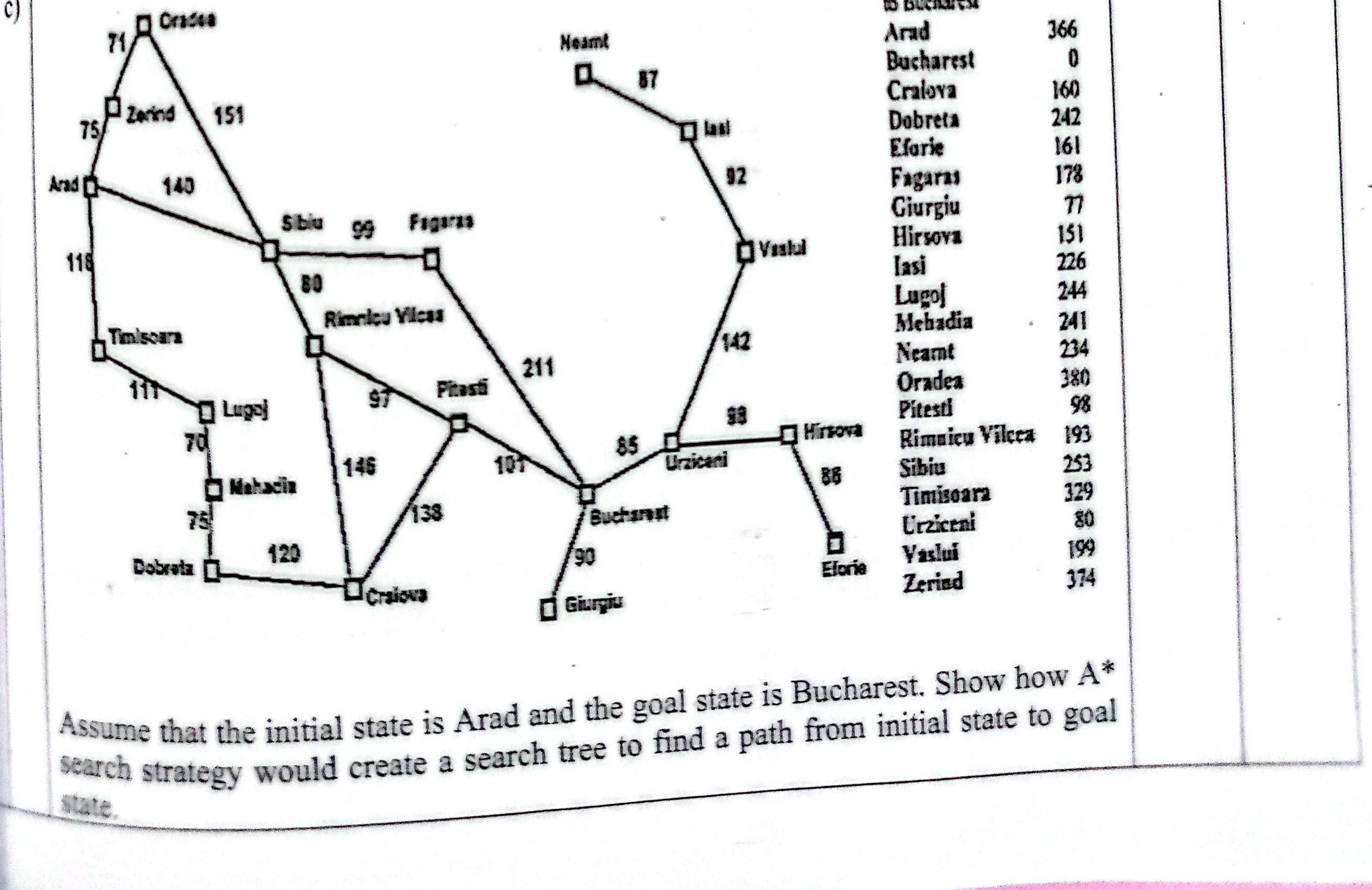
A* Search Tree from Arad to Bucharest (Romania Map):
Formula: \(f(n) = g(n) + h(n)\), where \(g(n)\) is exact path cost from Arad, and \(h(n)\) is straight-line distance to Bucharest from the table.
- Step 1: Expand Arad:
- \(g(\text{Arad}) = 0, h(\text{Arad}) = 366 \implies f(\text{Arad}) = 366\).
- Successors:
- Sibiu: \(g = 140, h = 253 \implies f = 393\)
- Timisoara: \(g = 118, h = 329 \implies f = 447\)
- Zerind: \(g = 75, h = 374 \implies f = 449\)
- Select minimum \(f\): Sibiu (\(f = 393\)).
- Step 2: Expand Sibiu:
- Successors:
- Fagaras: \(g = 140 + 99 = 239, h = 178 \implies f = 417\)
- Rimnicu Vilcea: \(g = 140 + 80 = 220, h = 193 \implies f = 413\)
- Oradea: \(g = 140 + 151 = 291, h = 380 \implies f = 671\)
- Frontier: Rimnicu Vilcea (413), Fagaras (417), Timisoara (447), Zerind (449), Oradea (671).
- Select minimum \(f\): Rimnicu Vilcea (\(f = 413\)).
- Successors:
- Step 3: Expand Rimnicu Vilcea:
- Successors:
- Pitesti: \(g = 220 + 97 = 317, h = 98 \implies f = 415\)
- Craiova: \(g = 220 + 146 = 366, h = 160 \implies f = 526\)
- Frontier: Pitesti (415), Fagaras (417), Timisoara (447), Zerind (449), Craiova (526), Oradea (671).
- Select minimum \(f\): Pitesti (\(f = 415\)).
- Successors:
- Step 4: Expand Pitesti:
- Successors:
- Bucharest: \(g = 317 + 101 = 418, h = 0 \implies f = 418\)
- Craiova: \(g = 317 + 138 = 455, h = 160 \implies f = 615\) (pruned, worse than existing).
- Frontier: Fagaras (417), Bucharest (418), Timisoara (447), Zerind (449), Craiova (526), Oradea (671).
- Select minimum \(f\): Fagaras (\(f = 417\)).
- Successors:
- Step 5: Expand Fagaras:
- Successors:
- Bucharest: \(g = 239 + 211 = 450, h = 0 \implies f = 450\) (inferior to existing path of 418).
- Frontier: Bucharest (418), Timisoara (447), Zerind (449), Bucharest (450), Craiova (526), Oradea (671).
- Select minimum \(f\): Bucharest (\(f = 418\)) → Goal reached!
- Successors:
Final Solution Path: \(\text{Arad} \to \text{Sibiu} \to \text{Rimnicu Vilcea} \to \text{Pitesti} \to \text{Bucharest}\)
Total Solution Cost: \(140 + 80 + 97 + 101 = \mathbf{418\text{ km}}\).
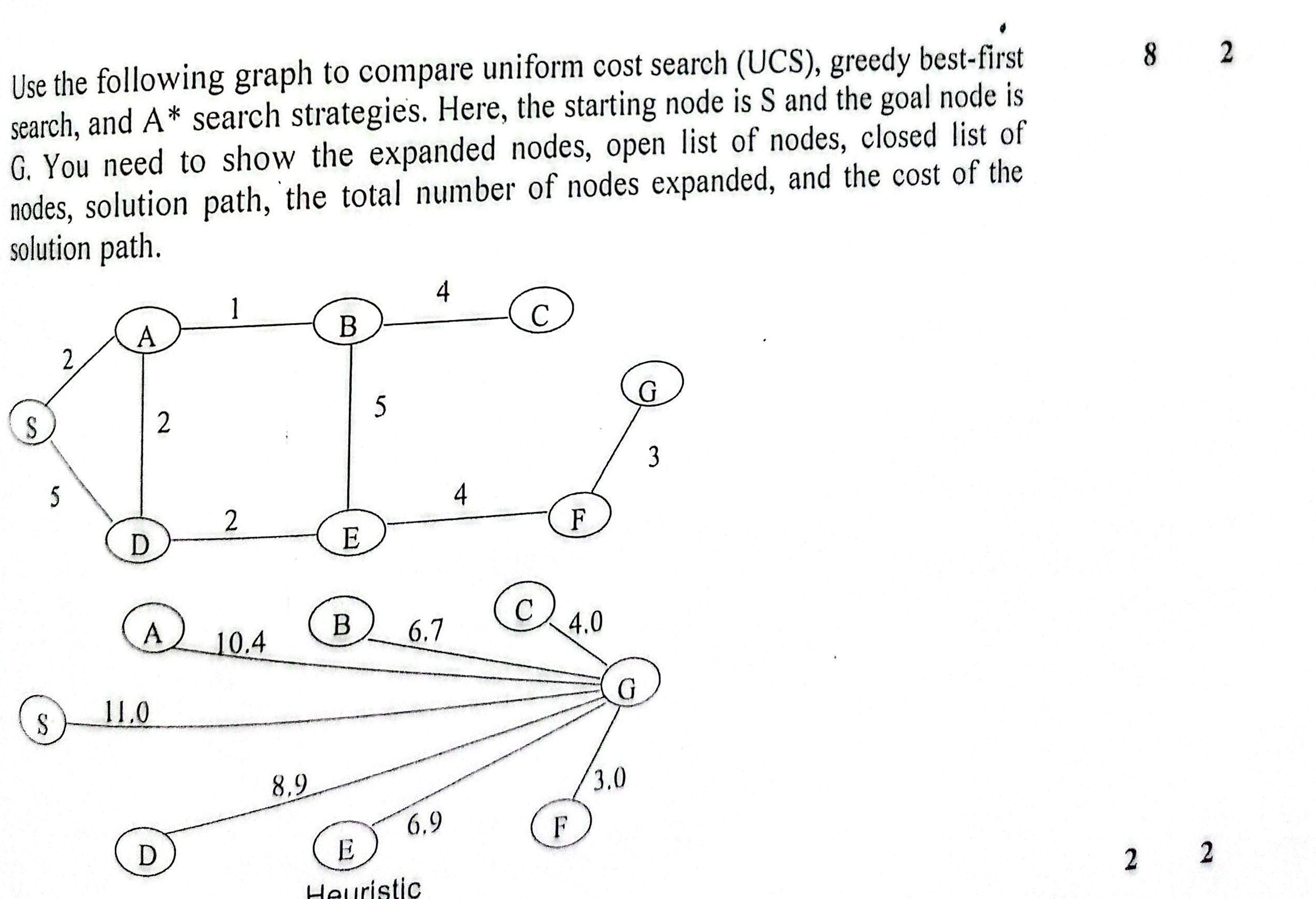
Graph Specifications: Start = \(S\), Goal = \(G\).
Arc Costs: \(S \to A: 2\), \(S \to D: 5\), \(A \to B: 1\), \(A \to D: 2\), \(B \to C: 4\), \(B \to E: 5\), \(D \to E: 2\), \(E \to F: 4\), \(F \to G: 3\).
Heuristics to \(G\): \(h(S)=11.0, h(A)=10.4, h(B)=6.7, h(C)=4.0, h(D)=8.9, h(E)=6.9, h(F)=3.0, h(G)=0\).
Strategy 1: Uniform Cost Search (UCS) — Orders by \(g(n)\):
| Step | Expanded Node | Open List (Frontier) | Closed List |
|---|---|---|---|
| 0 | — | \([S(0)]\) | \(\emptyset\) |
| 1 | \(S\) | \([A(2), D(5)]\) | \(\{S\}\) |
| 2 | \(A\) | \([B(3), D(4)]\) (via A, g(D)=4 beats 5) | \(\{S, A\}\) |
| 3 | \(B\) | \([D(4), C(7), E(8)]\) | \(\{S, A, B\}\) |
| 4 | \(D\) | \([E(6), C(7)]\) (via D, g(E)=6 beats 8) | \(\{S, A, B, D\}\) |
| 5 | \(E\) | \([C(7), F(10)]\) | \(\{S, A, B, D, E\}\) |
| 6 | \(C\) | \([F(10)]\) | \(\{S, A, B, D, E, C\}\) |
| 7 | \(F\) | \([G(13)]\) | \(\{S, A, B, D, E, C, F\}\) |
| 8 | \(G\) | Goal Reached! | \(\{S, A, B, D, E, C, F, G\}\) |
UCS Solution Path: \(S \to A \to D \to E \to F \to G\) • Cost: 13 • Total Nodes Expanded: 7.
Strategy 2: Greedy Best-First Search — Orders by \(h(n)\):
| Step | Expanded Node | Open List [Node(h)] | Closed List |
|---|---|---|---|
| 0 | — | \([S(11.0)]\) | \(\emptyset\) |
| 1 | \(S\) | \([D(8.9), A(10.4)]\) | \(\{S\}\) |
| 2 | \(D\) | \([E(6.9), A(10.4)]\) | \(\{S, D\}\) |
| 3 | \(E\) | \([F(3.0), B(6.7), A(10.4)]\) | \(\{S, D, E\}\) |
| 4 | \(F\) | \([G(0), B(6.7), A(10.4)]\) | \(\{S, D, E, F\}\) |
| 5 | \(G\) | Goal Reached! | \(\{S, D, E, F, G\}\) |
Greedy Solution Path: \(S \to D \to E \to F \to G\) • Cost: \(5 + 2 + 4 + 3 = 14\) • Total Nodes Expanded: 4.
Strategy 3: A* Search — Orders by \(f(n) = g(n) + h(n)\):
| Step | Expanded Node | Open List [Node(g + h = f)] | Closed List |
|---|---|---|---|
| 0 | — | \([S(0 + 11.0 = 11.0)]\) | \(\emptyset\) |
| 1 | \(S\) | \([A(2 + 10.4 = 12.4), D(5 + 8.9 = 13.9)]\) | \(\{S\}\) |
| 2 | \(A\) | \([B(3 + 6.7 = 9.7), D(4 + 8.9 = 12.9)]\) | \(\{S, A\}\) |
| 3 | \(B\) | \([C(7 + 4.0 = 11.0), D(4 + 8.9 = 12.9), E(8 + 6.9 = 14.9)]\) | \(\{S, A, B\}\) |
| 4 | \(C\) | \([D(4 + 8.9 = 12.9), E(8 + 6.9 = 14.9)]\) | \(\{S, A, B, C\}\) |
| 5 | \(D\) | \([E(6 + 6.9 = 12.9)]\) | \(\{S, A, B, C, D\}\) |
| 6 | \(E\) | \([F(10 + 3.0 = 13.0)]\) | \(\{S, A, B, C, D, E\}\) |
| 7 | \(F\) | \([G(13 + 0 = 13.0)]\) | \(\{S, A, B, C, D, E, F\}\) |
| 8 | \(G\) | Goal Reached! | \(\{S, A, B, C, D, E, F, G\}\) |
A* Solution Path: \(S \to A \to D \to E \to F \to G\) • Cost: 13 • Total Nodes Expanded: 7.
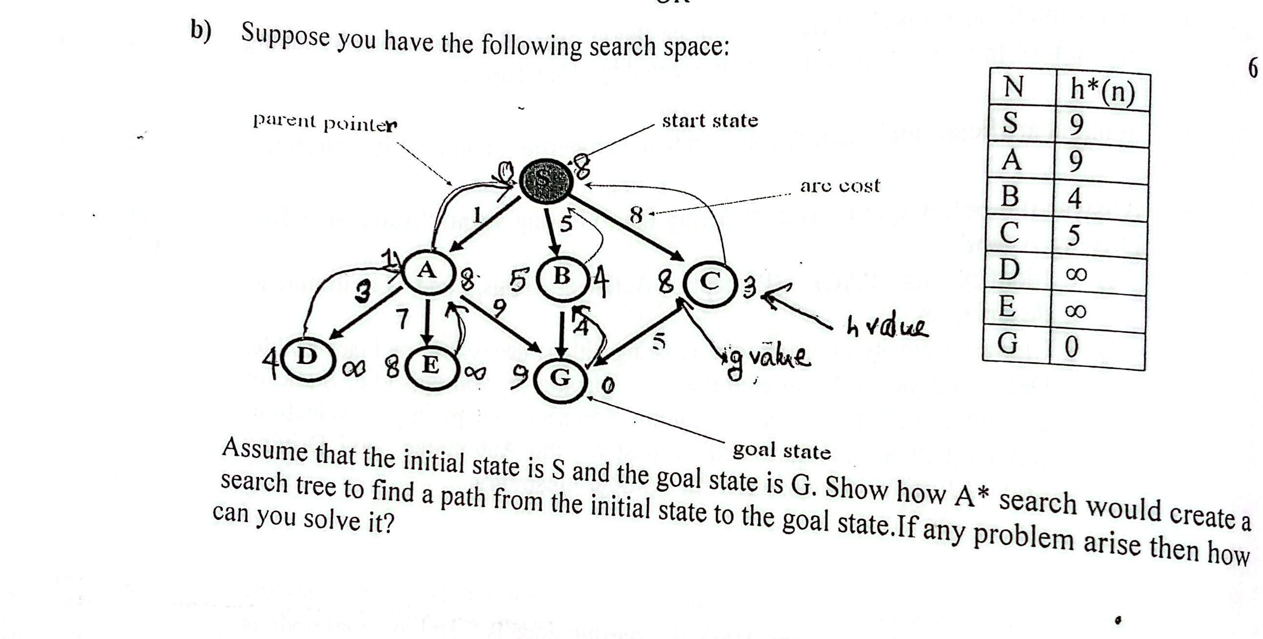
1. Search Tree Generation for A* Search Space:
Given the search graph with start \(S\) and goal \(G\), arc costs, parent pointers, and \(h^*(n)\) table: \(h^*(S)=9, h^*(A)=9, h^*(B)=4, h^*(C)=5, h^*(D)=\infty, h^*(E)=\infty, h^*(G)=0\).
Heuristics given in diagram: \(h(S)=8, h(A)=8, h(B)=4, h(C)=3, h(D)=\infty, h(E)=\infty, h(G)=0\).
2. Identifying the Inconsistency Problem:
Notice the edge between \(C\) and \(G\): Arc cost \(c(C, G) = 5\). Heuristic values: \(h(C) = 3\), but actual \(h^*(C) = 5\). However, on edge \(S \to C\): Arc cost is 8, \(h(S)=8, h(C)=3 \implies h(S) - h(C) = 5 \le 8\) (consistent). But on node \(A\): \(c(A, G) = 9\), \(h(A) = 8\). When expanding \(A\), if a node is closed and its heuristic drops steeply, standard graph search that permanently discards closed nodes will miss the optimal path!
3. How to Solve Any Problem That Arises (Fixing Graph Inconsistency):
- Node Reopening: In graph search, if a new path to a previously closed node \(n\) is discovered with a strictly lower \(g(n)\) value, reopen node \(n\) and re-insert it into the Frontier (Open List).
- Pathmax Equation: Enforce monotonicity along any step from \(n\) to child \(n'\) using: $$f(n') = \max(g(n') + h(n'), f(n))$$
- Consistency Adjustment: Modify the heuristic function so it obeys the triangle inequality: \(h(n) \le c(n, a, n') + h(n')\).
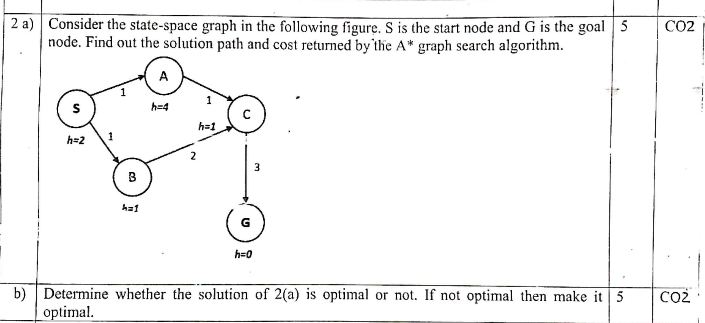
Part (a): Find Solution Path and Cost by A* Graph Search:
Graph Setup: Start \(S\), Goal \(G\). Arc costs: \(S \to A: 1, S \to B: 1, A \to C: 1, B \to C: 2, C \to G: 3\). Heuristics: \(h(S)=2, h(A)=4, h(B)=1, h(C)=1, h(G)=0\).
- Expand \(S\):
- Child \(A\): \(g=1, h=4 \implies f(A) = 5\).
- Child \(B\): \(g=1, h=1 \implies f(B) = 2\).
- Expand \(B\):
- Child \(C\): \(g = 1 + 2 = 3, h = 1 \implies f(C) = 4\).
- Expand \(C\):
- Child \(G\): \(g = 3 + 3 = 6, h = 0 \implies f(G) = 6\).
- Expand \(A\):
- Child \(C\): via \(A\), path cost would be \(g(C) = 1 + 1 = 2\). But in strict graph search without node reopening, \(C\) is already in Closed List and is DISCARDED!
- Expand \(G\): Goal reached with \(f(G) = 6\).
Returned Path: \(S \to B \to C \to G\) • Cost: 6.
Part (b): Determine whether the solution is optimal or not. If not, make it optimal:
1. Optimality Check: The solution \(S \to B \to C \to G\) (cost 6) is NOT OPTIMAL! The true optimal path is \(S \to A \to C \to G\) with cost \(1 + 1 + 3 = \mathbf{5} < 6\).
2. Cause of Failure: The heuristic is inconsistent (non-monotonic). Between node \(A\) and node \(C\):
$$h(A) - h(C) = 4 - 1 = 3 > c(A, C) = 1$$The estimated distance drops by 3 over an edge of cost 1, violating the triangle inequality \(h(A) \le c(A, C) + h(C) = 1 + 1 = 2\).
3. How to Make it Optimal:
- Algorithmic Fix: Enable Reopening of Closed Nodes in Graph Search. When expanding \(A\), since \(g_{new}(C) = 2 < g_{old}(C) = 3\), update \(g(C) = 2\) and re-insert \(C\) into Open List with \(f(C) = 2 + 1 = 3\). Then \(C\) expands to \(G\) with optimal cost \(2 + 3 = 5\).
- Heuristic Fix: Make the heuristic consistent by reducing \(h(A)\) to \(\le 2\) (e.g., set \(h(A) = 2\)). Then \(f(A) = 1 + 2 = 3 < f(C)=4\), so \(A\) expands before \(C\), finding the optimal path naturally.
Hill Climbing is an iterative optimization algorithm that begins with an arbitrary solution to a problem and continually attempts to find a better solution by making incremental changes. If a change produces an improvement, that improved state becomes the new baseline, and the process repeats until no further improvements can be found.
Hill climbing is classified as greedy local search with no backtracking because at each decision step, it greedily selects the neighbor with the highest objective evaluation value without maintaining an agenda or thinking ahead about subsequent moves. Once it steps to a new node, previous alternatives are discarded from memory.
ALGORITHM SimpleHillClimbing:
  1. Start: Begin at a random initial state on the problem landscape.
  2. Evaluate: Assess the objective value of the current state.
  3. Look Around: Generate neighboring states and evaluate their values.
  4. Can Improve: Determine if any neighbor has a higher objective value than current state.
  5. Move: If a superior neighbor exists, transition to that point.
  6. Repeat: Continue the iterative evaluation from the new state.
  7. No Improvement: If no neighbor is better than the current position, a peak has been reached.
  8. End: Terminate and return the peak as the best found solution.
        OBJECTIVE
        FUNCTION
           ▲                Global Maximum
           │                     /\
           │     Shoulder       /  \
           │    ┌────────┐     /    \
           │   /          \   /      \               Local Maximum
           │  /            \_/        \                   /\
           │ /                         \      Plateau    /  \
           │/                           \    ┌───────┐  /    \
           │                             \__/         \/      \____
           └────────────────────────────────────────────────────────► STATE SPACE
| Pitfall (Landscape Feature) | Mathematical Phenomenon | Algorithmic Consequence & Failure Mode |
|---|---|---|
| 1. Local Maxima (Slide 126) | A peak that is higher than each of its immediate neighboring states, but substantially lower than the global maximum. | Because all neighboring states evaluate to lower scores, the greedy condition \(\Delta \text{Value} > 0\) fails. The algorithm becomes permanently trapped, declaring premature convergence on an inferior solution. |
| 2. Ridges (Slide 127) | A sequence of local maxima joined together forming a narrow crest. The ridge slopes gently uphill, but single-variable coordinate moves step off the ridge into steep valleys. | Greedy orthogonal moves only see downhill directions. The search oscillates endlessly from side to side across the ridge, making virtually no forward progress. |
| 3. Plateau / Shoulder (Slide 128) | A flat region of the state space where all neighboring states share identical objective evaluation values. | • Flat Local Maximum: A flat plateau with no uphill exit. The algorithm cannot decide which direction leads upward. • Shoulder: A flat ledge from which upward progress is possible, but hill climbing may wander aimlessly or terminate prematurely before finding the uphill exit. |
| Advantages | Disadvantages |
|---|---|
| • Simple to understand and extraordinarily easy to implement. | • Not guaranteed to find the global optimal solution. |
| • Extremely lightweight: Requires \(O(1)\) space complexity (stores only current state). | • Highly sensitive to the choice of initial state; prone to local optima entrapment. |
| • Rapidly finds acceptable solutions if the heuristic landscape is smooth and well-behaved. | • Lacks a search history (no closed list), which can induce infinite loops or cycles. |
| • Well-suited for pure state optimization where path to goal is irrelevant. | • Completely ineffective on flat landscapes (plateaus) and jagged ridges. |
| Advanced Variant | Algorithmic Mechanism | How It Overcomes Classical Pitfalls |
|---|---|---|
| 1. Random-Restart Hill Climbing (Slide 130) | Executes multiple independent hill climbing searches, each beginning from a randomly generated initial state across the problem landscape. | Escapes Local Optima: If the probability of finding the global optimum from a random start is \(p\), the expected number of restarts is \(1/p\). With sufficient restarts, the probability of failure approaches zero: \(P(\text{failure after } k \text{ runs}) = (1 - p)^k \to 0\). |
| 2. Tabu Search (Slide 130) | Maintains a short-term memory list (the "Tabu List") containing recently visited states or operators, strictly forbidding the agent from revisiting them for a tenure of \(T\) steps. | Prevents Cycling & Escapes Plateaus: Forces the algorithm to accept non-improving (even downhill) moves when all neighbors are visited or plateaued, escaping local basins without looping. |
| 3. Local Beam Search (Slide 130) | Maintains \(k\) states simultaneously in memory rather than just one. At each iteration, all successors of all \(k\) states are generated. If any is a goal, it halts. Otherwise, it selects the top \(k\) best successors from the entire combined pool. | Information Sharing: Unlike \(k\) independent random restarts that run in isolation, Local Beam Search shares information across parallel trajectories. If one state discovers a promising uphill gradient, all \(k\) beams quickly converge toward that fertile region, bypassing plateaus and local maxima. |
Greedy Hill Climbing operates in \(O(1)\) memory, keeping only the single current state. It continually moves to the neighbor with the highest value.
       LOCAL MAXIMUM                    RIDGE                      PLATEAU
            /\                           / \                    _____________
           /  \                         /   \                  /                       /    \                       /  /\ \                /   (Zero           _____/      \_____                /  /  \ \              /   Gradient)        (Stuck below global peak)         (Oscillates across)    (Wanders aimlessly)
- Suitable Heuristic: \(h(n) =\) Total number of pairs of attacking queens. Goal state has \(h=0\).
- Total Successors: Any of 8 queens can move to 7 other squares in its column: \(8 \times 7 = \mathbf{56 \text{ successors}}\).
- How to Achieve 100% Success: Use Random-Restart Hill Climbing. Repeating independent trials from random initial states drives failure probability \((1-p)^k \to 0\).

1. The Hill Climbing Algorithm:
Hill Climbing is an iterative local search algorithm that continuously moves in the direction of increasing heuristic value (uphill) without maintaining a search tree or frontier. The algorithm terminates when it reaches a peak where no neighbor has a higher value.
function HILL-CLIMBING(problem) returns a state that is a local maximum
  current = problem.INITIAL-STATE
  loop do
    neighbor = HIGHEST-VALUED-SUCCESSOR(current)
    if VALUE(neighbor) <= VALUE(current) then return current.STATE
    current = neighbor
2. Why Greedy Hill Climbing Has Very Low Memory Requirements (Spring 2024 Q3.a):
Hill Climbing is a local search method that only maintains a single current state and its immediate successors in memory. Unlike BFS or A* which maintain exponential open lists (\(O(b^d)\)), Hill Climbing requires \(O(1)\) memory space.
3. The Three Main Drawbacks & How to Deal With Them:
- Local Maxima: A peak that is higher than all its neighboring states, but lower than the global maximum. The algorithm terminates prematurely thinking it found the optimum.
Remedy: Random-Restart Hill Climbing (conducting multiple runs from random initial states). - Ridges: A sequence of local maxima joined together sloping upward. Because successors are evaluated along single coordinates, all immediate moves go downhill off the ridge, stalling the search.
Remedy: Perform diagonal or macro-moves combining multiple operators. - Plateaux (Flat Local Maximum & Shoulders): A flat region where all adjacent states have identical evaluation values. The algorithm wanders aimlessly or gets stuck.
Remedy: Allow a limited number of sideways moves (e.g. up to 100 consecutive equal-value steps) or use Simulated Annealing.
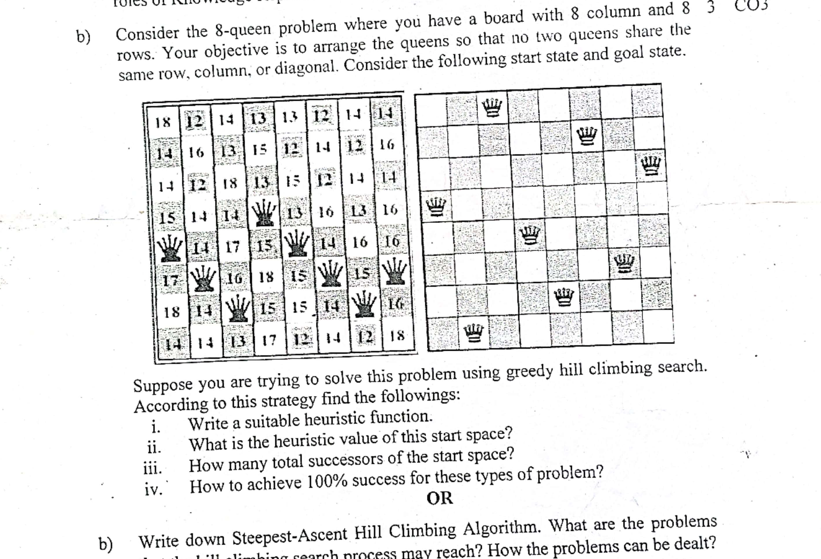
Analysis of the 8-Queens Grid Search:
i. Write a suitable heuristic function:
The standard heuristic function \(h(n)\) is defined as the number of pairs of queens attacking each other (either directly or indirectly along rows or diagonals). For a valid goal state, \(h(n) = 0\).
ii. What is the heuristic value of this start space?
By inspecting the board queens (one queen in each column) and counting all mutual attacks (e.g. queens sharing rows or diagonals), the heuristic value of the current configuration is \(h = \mathbf{17}\).
iii. How many total successors of the start space?
In the standard formulation of the 8-queens problem, each of the 8 columns has exactly 1 queen. In any single move, an operator shifts one queen to any other row within its column. Since each column has 8 rows, a queen has \(8 - 1 = 7\) available moves. Across all 8 columns:
$$\text{Total Successors} = 8 \times 7 = \mathbf{56 \text{ successor states}}.$$iv. How to achieve 100% success for these types of problem?
- Random-Restart Hill Climbing: Run the hill climbing algorithm repeatedly from uniformly distributed random initial board states. Since each restart has an independent probability of success \(p \approx 0.14\), the probability of finding the global optimum after \(k\) runs is \(1 - (1 - p)^k\). As \(k\) increases, success rate approaches 100%.
- Simulated Annealing: Allow probabilistic downhill moves with probability \(e^{\Delta E / T}\) to escape local maxima and plateaux.
- Min-Conflicts Local Search: A specialized CSP heuristic that resolves 8-queens in almost linear time \(O(n)\) with 100% reliability even for \(10,000,000\) queens!
Start State: Stack \(B \to C \to D \to E \to F \to G \to H \to A\). Goal: Stack \(A \to B \to C \to D \to E \to F \to G \to H\).
       START STATE                           GOAL STATE
       ┌───────────┐                        ┌───────────┐
       │     A     │                        │     H     │
       ├───────────┤                        ├───────────┤
       │     H     │                        │     G     │
       ├───────────┤                        ├───────────┤
       │     G     │                        │     F     │
       ├───────────┤                        ├───────────┤
       │     F     │                        │     E     │
       ├───────────┤                        ├───────────┤
       │     E     │                        │     D     │
       ├───────────┤                        ├───────────┤
       │     D     │                        │     C     │
       ├───────────┤                        ├───────────┤
       │     C     │                        │     B     │
       ├───────────┤                        ├───────────┤
       │     B     │                        │     A     │
       ┴───────────┴ (Table)                ┴───────────┴ (Table)
| Heuristic Type | Evaluation Method | Start State Score | Why it Fails or Succeeds |
|---|---|---|---|
| Local Heuristic (\(H_{\text{local}}\)) | \(+1\) if block rests on correct immediate block; \(-1\) if incorrect. | \(\mathbf{+4}\) | FAILS (Local Maximum): To fix bottom block \(B\), agent must dismantle stack. Dismantling decreases the local score; hill climbing refuses downhill steps and halts. |
| Global Heuristic (\(H_{\text{global}}\)) | Awards \(+n\) points only if the ENTIRE substack down to table is correct; \(-n\) if base is wrong. | \(\mathbf{-28}\) | SUCCEEDS: Start state gets severe negative score because base \(B\) is wrong. Clearing the table and placing \(A\) directly increases global score monotonically. |
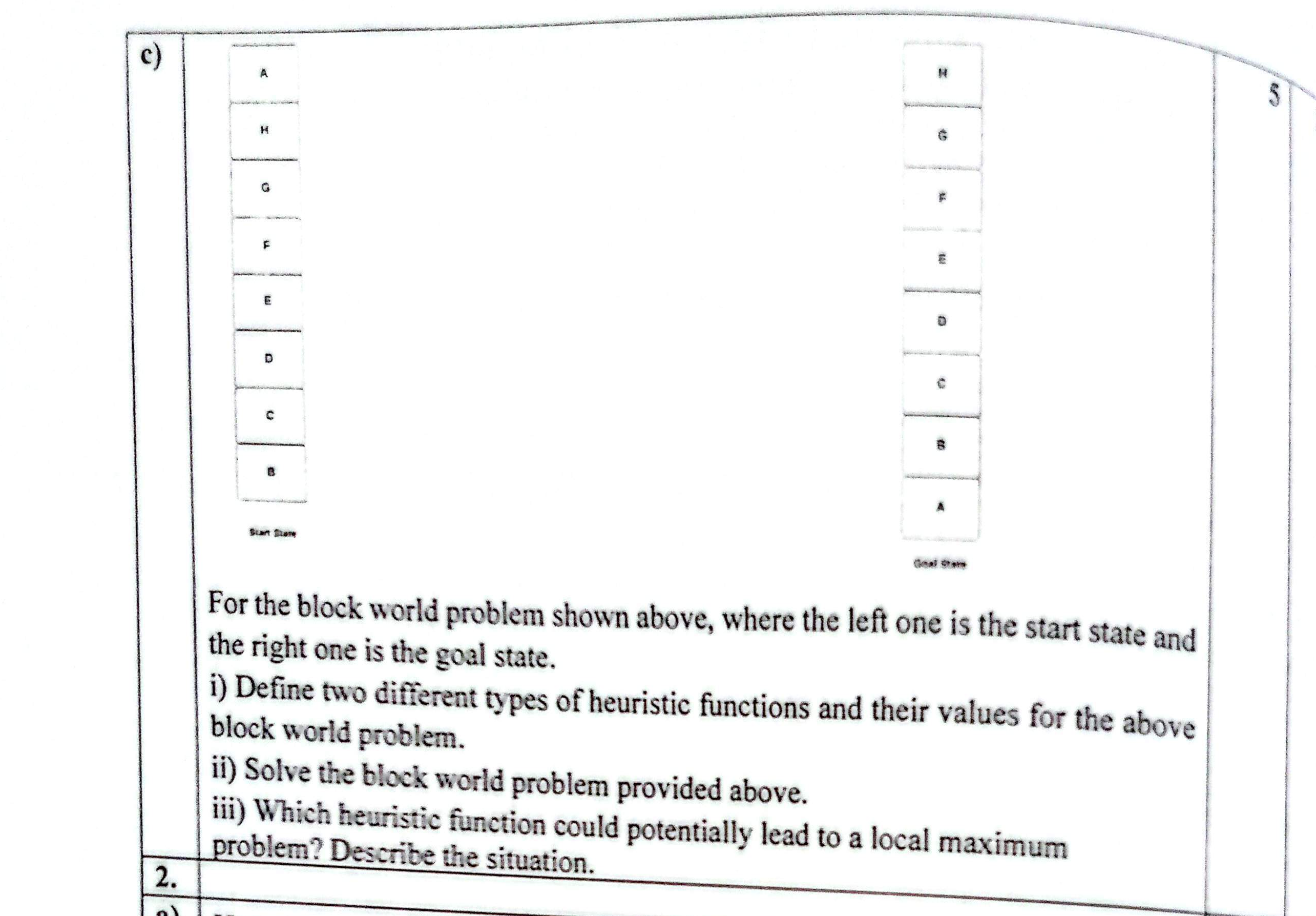
The Blocks World Problem (Local vs. Global Heuristic Functions):
Start State: Stack containing \([A \text{ on } H \text{ on } G \text{ on } F \text{ on } E \text{ on } D \text{ on } C \text{ on } B]\) resting on table.
Goal State: Stack containing \([H \text{ on } G \text{ on } F \text{ on } E \text{ on } D \text{ on } C \text{ on } B \text{ on } A]\) resting on table.
i. Two Different Types of Heuristic Functions & Their Values:
- Local Heuristic Function \(h_{local}\): Evaluates only individual support relationships.
- For each block: \(+1\) if it rests on the correct block as specified in the goal state; \(-1\) if it rests on an incorrect block.
- In the Start State: Every block rests on an incorrect block. For example, A is on H (incorrect), H is on G (correct in isolation, but below it everything is reversed). Local score is deeply negative.
- Global Heuristic Function \(h_{global}\): Evaluates the complete structural validity of the sub-stack beneath each block.
- For each block: \(+n\) (where \(n\) is depth/height) if the block and the entire sub-stack underneath it perfectly matches the goal state; \(-n\) if any block in the support structure beneath it is incorrect.
ii. Solving the Blocks World Problem:
To reach the goal from the start stack, block A must be at the very bottom on the table. Therefore, all blocks above A must be unstacked onto the table first, creating empty space, and then reassembled in ascending sequence: Table → A → B → C → D → E → F → G → H.
iii. Which Heuristic Function Leads to a Local Maximum? (Autumn 2022 Q1.b Proof):
The Local Heuristic Function inevitably leads to a Local Maximum!
Reasoning: To place block A on the table, the agent must pick up blocks (like H, G, etc.) and move them to the table. When moving block H from G to the table, the local heuristic sees that H was resting on G (\(+1\)) and is now on the table (\(-1\)), so the heuristic value decreases! Greedy hill climbing refuses to make moves that decrease heuristic score, so it stalls immediately in a local maximum without solving the problem.
In contrast, the Global Heuristic Function recognizes that H resting on an incorrect foundation is fundamentally flawed (\(-n\)). Dismantling the stack removes the large negative penalty, creating a strictly uphill gradient that successfully reaches the global goal state.
চার্লস ডারউইনের প্রাকৃতিক নির্বাচনের তত্ত্ব অনুযায়ী প্রকৃতিতে "Survival of the Fittest" নীতি কাজ করে। অর্থাৎ, যে প্রাণী পরিবেশের সাথে যত বেশি মানিয়ে নিতে পারে, সে বেঁচে থাকে এবং সন্তান জন্ম দিয়ে বংশবৃদ্ধি করে। দুর্বলরা ধীরে ধীরে হারিয়ে যায়।
কম্পিউটার সায়েন্স বা AI-তে কোনো জটিল সমস্যার সবচেয়ে সেরা সমাধান (Optimization/Best Solution) খুঁজে বের করতে প্রকৃতির ঠিক এই নিয়মটাই নকল করে Genetic Algorithm (GA) তৈরি করা হয়েছে।
প্রকৃতির প্রতিটি উপাদানের সাথে জেনেটিক অ্যালগরিদমের সরাসরি মিল রয়েছে:
| জীববিজ্ঞানের ধারণা (Biological Concept) | জেনেটিক অ্যালগরিদমে কী বোঝায় (GA Equivalent) | সহজ ব্যাখ্যা |
|---|---|---|
| Individual / Organism (জীব) | Candidate Solution (একটি সম্ভাব্য সমাধান) | যেকোনো একটি নির্দিষ্ট সমাধান। যেমন আগের ৮-কুইন সমস্যার একটি বিন্যাস 24748552। |
| Chromosome / DNA (ক্রোমোজোম) | Encoded String / Representation | সমাধানটির গাণিতিক বা কোডিং রূপ (যেমন বাইনারি বিট 10101 বা সংখ্যার সারি)। |
| Gene (জিন) | Single Feature / Character | ক্রোমোজোমের একটি মাত্র উপাদান বা সংখ্যা। |
| Population (জনসংখ্যা/গোষ্ঠী) | Set of Solutions (একগুচ্ছ সমাধান) | একসাথে থাকা অনেকগুলো সম্ভাব্য সমাধানের একটি সেট। |
| Fitness (টিকে থাকার যোগ্যতা) | Fitness Function / Objective Score | একটি সমাধান লক্ষ্য পূরণে কতটা ভালো তা পরিমাপ করার স্কোর। |
| Natural Selection (নির্বাচন) | Selection of Best Parents | বেশি ফিটনেস পাওয়া সমাধানগুলোকে প্যারেন্ট হিসেবে বেছে নেওয়া। |
| Reproduction / Crossover | Crossover Operator | দুটি প্যারেন্টের অংশ অদলবদল করে নতুন সমাধান (Child) তৈরি করা। |
| Mutation (জিনগত রূপান্তর) | Random Bit Flip / Small Change | বৈচিত্র্য ধরে রাখতে হঠাৎ দৈবচয়নভাবে কোনো জিনে ছোট পরিবর্তন আনা। |
জীববিজ্ঞানের প্রজন্ম তৈরির মতো GA নিচের ৫টি ধাপে কাজ করে:
Given: \(X_1 = 24748552, X_2 = 32752411, X_3 = 24415124, X_4 = 32543213\). Fitness = non-attacking pairs (\(\text{Max} = \binom{8}{2} = 28\)).
- Fitness of \(X_3\): Row conflicts = 5 attacks (three in row 4, two in row 1, two in row 2). Diagonal conflicts = 1 attack (\(Q_6(6,1)\) and \(Q_7(7,2)\)). Total attacks = \(5 + 1 = 6\). \(\mathbf{f(X_3) = 28 - 6 = 22}\).
- Fitness of \(X_4\): Row conflicts = 4 attacks. Diagonal conflicts = 6 attacks. Total attacks = \(4 + 6 = 10\). \(\mathbf{f(X_4) = 28 - 10 = 18}\).
- Fittest Individuals: \(X_1 (f=24)\) and \(X_2 (f=23)\).
- Crossover at 4th Point:
Parent 1: 2 4 7 4 | 8 5 5 2 Parent 2: 3 2 7 5 | 2 4 1 1 Offspring 1 = 24742411 Offspring 2 = 32758552 - Role of Mutation (Spring 2024 Exam): Prevents premature convergence. If all individuals share a common gene value at an index, crossover cannot produce alternatives. Mutation introduces fresh genetic diversity.
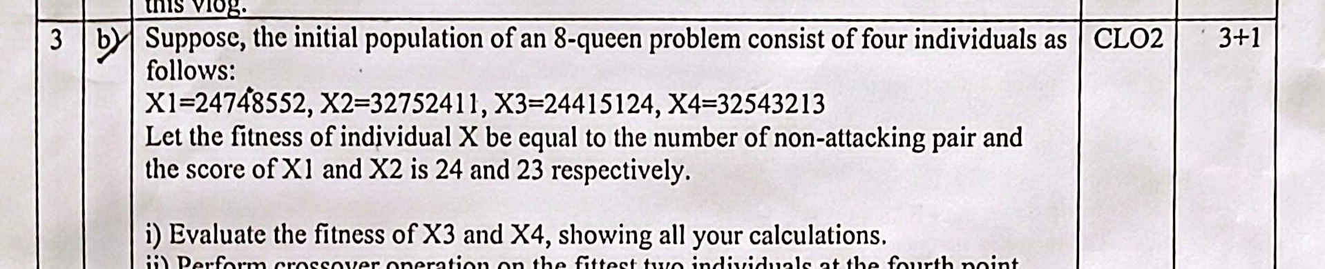
Genetic Algorithm on 8-Queens Problem:
Population chromosomes: \(X_1 = 24748552, X_2 = 32752411, X_3 = 24415124, X_4 = 32543213\).
Fitness formula: \(f(X) = \text{number of non-attacking pairs} = 28 - \text{attacking pairs}\).
Given: \(f(X_1) = 24\) (4 attacking pairs), \(f(X_2) = 23\) (5 attacking pairs).
i) Evaluate the fitness of \(X_3\) and \(X_4\) (showing all calculations):
For \(X_3 = [2, 4, 4, 1, 5, 1, 2, 4]\):
- Row conflicts (same digit):
- Digit 2 appears in col 1 and col 7 → 1 pair \((Q_1, Q_7)\).
- Digit 4 appears in col 2, col 3, col 8 → \(\binom{3}{2} = 3\) pairs: \((Q_2, Q_3), (Q_2, Q_8), (Q_3, Q_8)\).
- Digit 1 appears in col 4 and col 6 → 1 pair \((Q_4, Q_6)\).
- Total Row Conflicts: \(1 + 3 + 1 = 5\).
- Diagonal conflicts (\(|r_i - r_j| == |c_i - c_j|\)):
- \(Q_2(4)\) at col 2 and \(Q_4(1)\) at col 4: \(|4 - 1| = 3, |2 - 4| = 2 \implies\) no.
- \(Q_5(5)\) at col 5 and \(Q_6(1)\) at col 6: \(|5 - 1| = 4, |5 - 6| = 1 \implies\) no.
- \(Q_4(1)\) at col 4 and \(Q_5(5)\) at col 5: \(|1 - 5| = 4, |4 - 5| = 1 \implies\) no.
- \(Q_1(2)\) at col 1 and \(Q_2(4)\) at col 2: \(|2 - 4| = 2, |1 - 2| = 1 \implies\) no.
- \(Q_6(1)\) at col 6 and \(Q_7(2)\) at col 7: \(|1 - 2| = 1, |6 - 7| = 1 \implies\) 1 diagonal conflict \((Q_6, Q_7)\).
- \(Q_5(5)\) at col 5 and \(Q_8(4)\) at col 8: \(|5 - 4| = 1, |5 - 8| = 3 \implies\) no.
- \(Q_7(2)\) at col 7 and \(Q_8(4)\) at col 8: \(|2 - 4| = 2, |7 - 8| = 1 \implies\) no.
- \(Q_3(4)\) at col 3 and \(Q_5(5)\) at col 5: \(|4 - 5| = 1, |3 - 5| = 2 \implies\) no.
- \(Q_2(4)\) at col 2 and \(Q_5(5)\) at col 5: \(|4 - 5| = 1, |2 - 5| = 3 \implies\) no.
- Total attacking pairs in \(X_3 = 5 \text{ (row)} + 1 \text{ (diag)} = 6\).
- Fitness of \(X_3\) = \(28 - 6 = \mathbf{22}\).
For \(X_4 = [3, 2, 5, 4, 3, 2, 1, 3]\):
- Row conflicts:
- Digit 3 appears in col 1, col 5, col 8 → \(\binom{3}{2} = 3\) pairs.
- Digit 2 appears in col 2, col 6 → 1 pair.
- Total Row Conflicts: \(3 + 1 = 4\).
- Diagonal conflicts:
- \(Q_1(3)\) at col 1 and \(Q_2(2)\) at col 2: \(|3 - 2| = 1, |1 - 2| = 1 \implies\) 1 conflict.
- \(Q_3(5)\) at col 3 and \(Q_4(4)\) at col 4: \(|5 - 4| = 1, |3 - 4| = 1 \implies\) 1 conflict.
- \(Q_4(4)\) at col 4 and \(Q_5(3)\) at col 5: \(|4 - 3| = 1, |4 - 5| = 1 \implies\) 1 conflict.
- \(Q_5(3)\) at col 5 and \(Q_6(2)\) at col 6: \(|3 - 2| = 1, |5 - 6| = 1 \implies\) 1 conflict.
- \(Q_6(2)\) at col 6 and \(Q_7(1)\) at col 7: \(|2 - 1| = 1, |6 - 7| = 1 \implies\) 1 conflict.
- \(Q_7(1)\) at col 7 and \(Q_8(3)\) at col 8: \(|1 - 3| = 2, |7 - 8| = 1 \implies\) no.
- \(Q_3(5)\) at col 3 and \(Q_7(1)\) at col 7: \(|5 - 1| = 4, |3 - 7| = 4 \implies\) 1 conflict.
- Total attacking pairs in \(X_4 = 4 \text{ (row)} + 6 \text{ (diag)} = 10\).
- Fitness of \(X_4\) = \(28 - 10 = \mathbf{18}\).
ii) Perform Crossover on the Fittest Two Individuals at the Fourth Point:
The fitness values are: \(f(X_1) = 24, f(X_2) = 23, f(X_3) = 22, f(X_4) = 18\).
The fittest two individuals are \(X_1 = 24748552\) and \(X_2 = 32752411\).
Performing 1-point crossover at the 4th point (after the 4th digit):
Parent 1 (X1): [ 2  4  7  4 | 8  5  5  2 ]
Parent 2 (X2): [ 3  2  7  5 | 2  4  1  1 ]
------------------------------------------
Offspring Child 1: [ 2  4  7  4 | 2  4  1  1 ] = 24742411
Offspring Child 2: [ 3  2  7  5 | 8  5  5  2 ] = 32758552

1. Genetic Algorithms in Contrast to Biological Concepts:
Genetic Algorithms (GA) are stochastic search and optimization heuristics inspired by Charles Darwin's theory of natural evolution.
| Biological Evolution Concept | Genetic Algorithm Computational Equivalent |
|---|---|
| Chromosome | A candidate solution encoded as a string/vector of bits, integers, or characters. |
| Gene | A single position or variable in the chromosome string (e.g. column row in 8-queens). |
| Individual / Organism | A single point in the search space. |
| Population | A set of active candidate solutions evaluated simultaneously. |
| Natural Selection ("Survival of the Fittest") | Selection operator (Roulette Wheel, Tournament) based on Fitness Function. |
| Crossover / Reproduction | Recombination operator swapping genetic material between two fit parents to produce offspring. |
| Mutation | Random alteration of individual genes to preserve genetic diversity. |
2. Why the Mutation Step Increases Diversification (Spring 2024 Q3.a):
Over successive generations, crossover solely recombines existing alleles present in the initial population. Without mutation, if an essential bit value is missing from the entire population, crossover can never generate it, leading to premature convergence and entrapment in sub-optimal local peaks. Mutation introduces brand new, random genetic variations, effectively exploring uncharted regions of the search space and preventing genetic stagnation.
সাধারণ গ্রাফ (OR Graph) বনাম সমস্যা বিভাজন (Problem Reduction):
সাধারণ সার্চ অ্যালগরিদমগুলো (যেমন BFS, DFS, UCS, বা A*) কাজ করে OR Graph-এ।
OR Graph-এর অর্থ: একটি কাজ করার একাধিক বিকল্প পথ থাকে এবং যেকোনো একটি পথে গন্তব্যে পৌঁছালেই কাজ শেষ। যেমন: স্কুলে যাওয়ার জন্য হেঁটে যাওয়া OR বাসে যাওয়া। যেকোনো একটি বেছে নিলেই চলে।
কিন্তু বাস্তব জীবনের বহু জটিল সমস্যাকে একাধিক ছোট ছোট উপ-সমস্যায় (Sub-problems) ভাগ করতে হয় (যাকে বলে Problem Reduction বা সমস্যা বিভাজন)। সেখানে এমন পরিস্থিতি আসে যেখানে সব কটি উপ-সমস্যাই সমাধান করতে হয়।
লক্ষ্য: একটি ফোন সংগ্রহ করা (Acquire a Phone)
- বিকল্প ১ (OR পথ): ফোন চুরি করা (Steal Phone)। এটি নিজে একাই কাজ শেষ করে দেয় (যদিও অনৈতিক)।
- বিকল্প ২ (AND পথ): বৈধভাবে ফোন নেওয়া। বৈধভাবে ফোন নিতে হলে আপনাকে টাকা উপার্জন করতে হবে (Earn Money) AND সেই টাকা দিয়ে ফোন কিনতে হবে (Purchase Phone)।
এখানে শুধু টাকা কামিয়ে বসে থাকলে ফোন আসবে না, আবার টাকা ছাড়া ফোন কেনার দোকানে গেলেও ফোন দেবে না। লক্ষ্য পূরণ করতে হলে দুটো কাজই সম্পন্ন করতে হবে।
                                Goal: Acquire a Phone
                                   /            \
                        (OR Arc)  /              \  (AND Arc)
                                 /                \
                         Steal Phone         ┌─────────────┐
                         (Alternative 1)     │ Earn Money  │
                                             │     AND     │
                                             │Purchase Phone│
                                             └─────────────┘
যে গ্রাফে এরকম বিকল্প পথ (OR) এবং একাধিক কাজের যৌথ বাধ্যবাধকতা (AND) দুটিই থাকে, তাকে AND-OR Graph বলে। সাধারণ A* কেবল একটি একক সরল পথ (Single Path) খোঁজে, কিন্তু AND-OR গ্রাফে আমাদের খুঁজতে হয় একটি সমাধান গাছ (Solution Subtree/Sub-graph)। এই কারণেই এখানে সাধারণ A* ব্যর্থ হয় এবং প্রয়োজন হয় AO* (AND-OR A*) অ্যালগরিদম।
কোনো নোড \(n\)-এর খরচ হিসাবের সাধারণ নিয়ম:
OR শাখার জন্য:
যদি নোড \(n\) থেকে কেবল একটি পথ বেছে নেওয়ার সুযোগ থাকে (যেমন শিশু \(m\)):
$$\text{Cost} = c(n, m) + h(m)$$(এখানে \(c\) হলো এজ বা রাস্তার খরচ, আর \(h\) হলো শিশু নোডের আনুমানিক বা হিউরিস্টিক খরচ)
AND শাখার জন্য:
যদি নোড \(n\) থেকে একাধিক নোডকে একসঙ্গে সমাধান করতে হয় (যেমন শিশু \(m_1, m_2, \dots, m_k\)):
$$\text{Cost} = \sum [c(n, m_i) + h(m_i)]$$(সহজ কথায়: সবকটি শাখার রাস্তার খরচ এবং তাদের নিজ নিজ হিউরিস্টিক মানগুলো যোগ করতে হবে)
স্লাইডের গাঠনিক ট্রিতে প্রতিটি এজের (রাস্তার) খরচ ধরা হয়েছে \(c = 1\)।
                                     [ A ]
                                    /  |  \
                                   /   |   \  (AND Arc connecting C & D)
                             1    /  1 |    \ 1
                                 /     |     \
                              [ B ]  [ C ]  [ D ]
                              (4)     (2)    (3)
                              / \     / \     │
                           1 / 1 \ 1 / 1 \    │ 1
                            /     \ /     \   │
                          [E]    [F][G]  [H, I][J]
                          (6)    (8)(2)  (1)(1)(1)
প্রাথমিক নোডগুলোর দেওয়া মান: \(h(B) = 4, \quad h(C) = 2, \quad h(D) = 3\)
পাতার নোডগুলো (Leaf nodes):
\(h(E) = 6\), \(h(F) = 8\), \(h(G) = 2\), \(h(H) = 1, \quad h(I) = 1\), \(h(J) = 1\)
ধাপ ১: নোড B-এর উপবৃক্ষ মূল্যায়ন (OR Branch)
নোড \(B\) থেকে নিচে দুটি বিকল্প রাস্তা আছে (OR):
- পথ ১ (\(B \to E\)): $$\text{Cost} = c(B, E) + h(E) = 1 + 6 = 7$$
- পথ ২ (\(B \to F\)): $$\text{Cost} = c(B, F) + h(F) = 1 + 8 = 9$$
যেহেতু \(B\) একটি OR নোড, আমরা সর্বনিম্ন খরচটি নেব:
$$\min(7, 9) = 7$$আপডেট: \(B\)-এর হিউরিস্টিক মান আগে ছিল \(4\), তা পরিবর্তিত হয়ে এখন হলো \(7\) (\(h(B) = 7\))।
যদি \(A\) থেকে \(B\)-তে যাওয়া হয়, তবে মোট খরচ দাঁড়ায়:
$$\text{Cost}(A \to B) = c(A, B) + h(B) = 1 + 7 = 8$$ধাপ ২: AND শাখা (C এবং D)-এর উপবৃক্ষ মূল্যায়ন
\(A\) থেকে ডানে যে শাখাটি নেমেছে, সেটি একটি AND শাখা। অর্থাৎ \(C\) এবং \(D\) উভয়কেই সমাধান করতে হবে।
(ক) নোড C মূল্যায়ন:
\(C\) থেকে দুটি পথ আছে:
- বিকল্প ১ (\(C \to G\) [OR branch]): $$\text{Cost} = c(C, G) + h(G) = 1 + 2 = 3$$
- বিকল্প ২ (\(C \to H \text{ AND } I\) [AND branch]):
এখানে \(H\) ও \(I\) দুটোই করতে হবে: $$\text{Cost} = [c(C, H) + h(H)] + [c(C, I) + h(I)] = (1 + 1) + (1 + 1) = 2 + 2 = 4$$
\(C\)-এর জন্য সেরা বিকল্প হলো \(\min(3, 4) = 3\) (অর্থাৎ \(G\)-এর দিকে যাওয়া)।
আপডেট: \(C\)-এর মান আগে ছিল \(2\), তা বেড়ে হলো \(3\) (\(h(C) = 3\))।
(খ) নোড D মূল্যায়ন:
\(D\) থেকে একটিই পথ আছে (\(D \to J\)):
$$\text{Cost} = c(D, J) + h(J) = 1 + 1 = 2$$আপডেট: \(D\)-এর মান আগে ছিল \(3\), তা সংশোধিত হয়ে হলো \(2\) (\(h(D) = 2\))।
(গ) \(A \to (C, D)\) এর সমন্বিত AND খরচ:
যেহেতু \(C\) এবং \(D\) দুটোই AND দিয়ে যুক্ত:
$$\text{Cost}(A \to C, D) = [c(A, C) + h(C)] + [c(A, D) + h(D)] = (1 + 3) + (1 + 2) = 4 + 3 = 7$$ধাপ ৩: রুট নোড A-তে চূড়ান্ত সিদ্ধান্ত গ্রহণ
এখন রুট নোড \(A\)-এর সামনে দুটি প্রধান বিকল্প:
- বাম দিকের OR পথ (\(B\)): মোট খরচ = \(8\)
- ডান দিকের AND পথ (\(C\) এবং \(D\)): মোট খরচ = \(7\)
সিদ্ধান্ত: যেহেতু \(7 < 8\), তাই AO* অ্যালগরিদম ডানদিকের AND শাখাকে (\(C\) ও \(D\)) সর্বোত্তম হিসেবে চিহ্নিত করবে।
ALGORITHM AO* (StartNode):
  1. Initialize graph G with the StartNode.
  2. WHILE the partial solution graph contains non-terminal leaf nodes:
       a. Traverse marked best branches to find a non-terminal node n.
       b. Expand n: generate all successors (creating OR / AND arcs) and initialize their heuristics.
       c. Create a set S containing n and all its ancestors in G.
       d. WHILE S is not empty:
            - Remove a node p from S that has no descendants in S.
            - Recompute cost of each branch from p:
                For OR branch: cost = c(p, child) + h(child)
                For AND branch: cost = SUM [c(p, child_i) + h(child_i)]
            - Update h(p) to the minimum branch cost and mark the best branch.
            - If h(p) changed, add parents of p to S.
  3. Terminate when the StartNode is marked terminal (fully solved).
| Property | AO* Algorithm Characteristics (Slides 122–123) |
|---|---|
| Completeness | Complete: Guaranteed to find a solution graph if one exists in a finite graph. |
| Optimality | Optimal: Guaranteed to find the optimal cost solution tree if the heuristic function \(h(n)\) is admissible (\(h(n) \le h^*(n)\)) and consistent (satisfies triangle inequality). |
| Memory & Complexity | Consumes substantial memory because it must store the entire partially expanded solution graph and ancestors to perform bottom-up cost revisions. |
Means-Ends Analysis (MEA) is a classical AI problem-solving strategy that combines forward and backward reasoning to solve complex, high-dimensional problems. First introduced in Allen Newell and Herbert Simon's General Problem Solver (GPS, 1957), MEA focuses its computational effort on identifying significant differences between the current state and the goal state, and selecting operators explicitly designed to reduce those specific differences.
In many real-world tasks, the operator that eliminates the largest difference between the current state and the goal cannot be applied immediately because its preconditions are not satisfied in the current state.
Operator Subgoaling is the process within MEA of setting up intermediate sub-goals whose sole purpose is to transform the current state into one where the blocked operator's preconditions are satisfied. Once the sub-goal is achieved, the primary operator is executed.
- Identify Differences: Compare current state \(S_{current}\) with goal state \(S_{goal}\) and enumerate all discrepancies.
- Set Sub-goals: Formulate intermediate sub-goals targeted at reducing the most significant identified difference.
- Find Operators: Query the domain operator library for actions capable of reducing the selected difference.
- Apply Operators (or Subgoal): If preconditions are met, apply the operator to yield a new state. If preconditions are violated, initiate Operator Subgoaling to remove the blocking constraints.
- Iterate: Repeat until zero differences remain between the current state and the goal state.
Consider the visual problem given in the course lecture slides:
    INITIAL STATE                                      GOAL STATE
    ┌───────────────────────────┐                      ┌───────────────────────────┐
    │                       ●   │                      │                    ▲      │
    │                    (dot)  │                      │                 (large    │
    │       ┌───────┐           │                      │       ┌───────┐  triangle)│
    │       │   ▲   │           │                      │       │       │           │
    │       │(small)│           │                      │       │(empty)│           │
    │       └───────┘           │                      │       └───────┘           │
    │        circle             │                      │        circle             │
    └───────────────────────────┘                      └───────────────────────────┘
Difference Analysis: Comparing Initial State and Goal State reveals 3 discrepancies:
- Difference 1: A black dot is present in the initial state but absent in the goal state.
- Difference 2: The triangle is inside the circle in the initial state, but outside in the goal state.
- Difference 3: The triangle is small in the initial state, but large in the goal state.
Step 1: Apply Delete Operator (Slide 133)
The first difference is the unwanted dot symbol. MEA applies the Delete operator to remove the dot.
Resulting State: Circle with small triangle inside, dot is gone.
Step 2: Apply Move Operator (Slide 134)
Comparing the new state with the goal state reveals the triangle is inside the circle. MEA applies the Move operator to reposition the small triangle to the top-right outside the circle.
Resulting State: Circle is empty; small triangle is located outside in the upper-right corner.
Step 3: Apply Expand Operator (Slide 135)
Comparing with the goal state reveals only one remaining difference: the size of the triangle. MEA selects and executes the Expand operator, enlarging the triangle.
Final State: Circle is empty; large triangle is outside in the upper-right. Goal State Achieved!
The Water Jug Problem is a classic computer science and AI benchmark used to demonstrate problem formulation, state-space search, and Means-Ends Analysis.
- Jug X: Capacity of 5 Liters.
- Jug Y: Capacity of 3 Liters.
- Water Supply: An endless tap/pump to fill jugs and a drain to empty them.
- Constraints: Neither jug has any intermediate measurement markings. You can only fill completely, empty completely, or pour from one jug to another until either the source jug is empty or the receiving jug is full.
- Goal: Measure out exactly 4 Liters in Jug X.
• State Representation: An ordered pair \((x, y)\) where \(x \in \{0, 1, 2, 3, 4, 5\}\) denotes liters in Jug X, and \(y \in \{0, 1, 2, 3\}\) denotes liters in Jug Y.
• Initial State: \((0, 0)\)
• Goal State: \((4, y)\) where \(y\) can be any value.
| Step | Action / Operator Executed | State \((x, y)\) | Physical Reasoning & Rule Applied |
|---|---|---|---|
| 0 | Initial Configuration | (0, 0) |
Both Jug X (5L) and Jug Y (3L) start empty. |
| 1 | Fill Jug X (5L) to full capacity | (5, 0) |
Tap fills Jug X completely with 5 Liters. |
| 2 | Pour water from Jug X into Jug Y until Y is full | (2, 3) |
Jug Y takes 3L from X. Jug X is left with \(5 - 3 = 2\text{L}\). |
| 3 | Empty Jug Y into the drain | (2, 0) |
Jug Y is dumped out; Jug X retains its 2 Liters. |
| 4 | Pour remaining 2L from Jug X into Jug Y | (0, 2) |
All 2L transferred to Y. Jug X is now empty; Y has 2L (capacity for 1L more). |
| 5 | Fill Jug X (5L) completely from tap | (5, 2) |
Jug X is filled to 5L; Jug Y still holds 2L. |
| 6 | Pour from Jug X into Jug Y until Y is full | (4, 3) |
Jug Y has 2L, so it can only take \(3 - 2 = 1\text{L}\). Pouring 1L from X leaves exactly \(5 - 1 = \mathbf{4\text{ Liters}}\) in Jug X! |
Jug X now holds exactly 4 Liters. The minimal production system reaches the goal in 6 transitions: \((0,0) \to (5,0) \to (2,3) \to (2,0) \to (0,2) \to (5,2) \to (4,3)\).
Game Playing, CSP & Optimization
The Minimax Algorithm is a specialized recursive backtracking search algorithm used in two-player zero-sum games of perfect information (such as Chess, Checkers, and Tic-Tac-Toe) to determine the optimal strategy for the players.
• MAX Player: Seeks moves that maximize the utility/score. Initialized with \(-\infty\) as its worst-case starting bound.
• MIN Player: Seeks moves that minimize the MAX player's outcome. Initialized with \(+\infty\) as its worst-case starting bound.
• Mechanism: Computes the minimax decision for the current state using a depth-first search of the complete game tree.
                        MAX (A) = 4
                       /           \
                      /             \
               MIN (B) = 4       MIN (C) = -3
                 /     \           /     \
                /       \         /       \
          MAX (D)=4  MAX (E)=6 MAX (F)=-3 MAX (G)=7
            /   \      /   \     /   \      /   \
           H     I    J     K   L     M    N     O
          -1     4    2     6  -3    -5    0     7
Step-by-Step Bottom-Up Value Propagation:
- Level 2 (MAX Nodes):
- Node D: \(\max(H, I) = \max(-1, 4) = \mathbf{4}\).
- Node E: \(\max(J, K) = \max(2, 6) = \mathbf{6}\).
- Node F: \(\max(L, M) = \max(-3, -5) = \mathbf{-3}\).
- Node G: \(\max(N, O) = \max(0, 7) = \mathbf{7}\).
- Level 1 (MIN Nodes):
- Node B: \(\min(D, E) = \min(4, 6) = \mathbf{4}\).
- Node C: \(\min(F, G) = \min(-3, 7) = \mathbf{-3}\).
- Level 0 (Root MAX Node A): $$\text{Value}(A) = \max(B, C) = \max(4, -3) = \mathbf{4}$$
Minimax Decision: MAX should move to child B, guaranteeing a payoff of at least 4 regardless of MIN's optimal play.
| Property (Slide 157) | Evaluation & Real-World Complexity |
|---|---|
| Completeness | Complete: Guaranteed to find a solution if the game tree is finite. |
| Optimality | Optimal: Provably finds the optimal strategy against an optimal adversary. |
| Time Complexity | \(O(b^m)\): Where \(b\) is the legal branching factor and \(m\) is the maximum game depth. |
| Space Complexity | \(O(b \cdot m)\): Generates nodes via Depth-First Search; only the current path is retained in memory. |
| Core Limitation | In complex board games like chess (\(b \approx 35, m \approx 80\)), evaluating \(35^{80} \approx 10^{123}\) states is completely impossible. This demands heuristic depth cutoffs and Alpha-Beta Pruning. |
Alpha-Beta Pruning is an optimization for the minimax algorithm that eliminates branches of the game tree that provably cannot influence the final decision, without altering the optimal outcome.
• \(\alpha\) (Alpha): The best (highest) value that the MAX player can guarantee at the current level or above. Initialized to \(-\infty\).
• \(\beta\) (Beta): The best (lowest) value that the MIN player can guarantee at the current level or above. Initialized to \(+\infty\).
• When to Prune: A branch is pruned whenever: $$\mathbf{\alpha \ge \beta}$$ Because the minimizer would never allow the game to enter a state yielding a value worse than what the maximizer has already guaranteed elsewhere!
Consider the deep 4-level adversarial tree with alternating MAX/MIN levels from course lecture slides 159–160:
Level 0 (MAX):                [ Root: α=2, β=∞ ]
                             /                  \
Level 1 (MIN):       [ Node 1: α=-∞, β=2 ]       [ Node 2: α=2, β=2 ]  ──► PRUNED SUBTREE!
                     /                  \
Level 2 (MAX):  [ α=-∞, β=5 ]      [ α=2, β=5 ]
                /           \      /          \
Level 3 (MIN): [5, 12]     [7, 3] [2, 8]     [18, 1] ...
Cutoff Mechanics:
- When evaluating the left subtree, the minimum node returns \(5\), setting \(\alpha = 5\). Then the next branch encounters a leaf value of \(3\). Because MIN chooses the minimum, this node cannot exceed \(3\). Since \(3 < 5\) (i.e. \(\beta \le \alpha\)), the sibling branches are pruned!
- At Root MAX, \(\alpha\) is updated to \(2\).
- When the search moves to the right primary subtree, a branch reveals a value \(\le 2\). Because \(\beta \le \alpha\) (\(2 \le 2\)), the entire remaining branch of Node 2 is pruned immediately!
Benefits of Alpha-Beta Pruning (Slide 161):
- Efficiency: In the best-case (perfect move ordering), the effective branching factor is reduced to \(\sqrt{b}\), reducing time complexity to \(O(b^{m/2})\)! This effectively doubles the searchable depth in competitive chess engines.
- Optimality Preserved: The final decision is mathematically identical to running full exhaustive minimax.
In two-player zero-sum games, MAX tries to maximize utility while MIN tries to minimize it. Time complexity is \(O(b^m)\).
Alpha-Beta Pruning: Maintains \(\alpha\) (best value for MAX) and \(\beta\) (best value for MIN). Prunes whenever \(\mathbf{\alpha \ge \beta}\). With perfect move ordering, time complexity improves to \(O(b^{m/2})\).
                                ( a )  MAX  [Root]
                              /                                   /                               ( b ) MIN           ( h ) MIN
                   /         \         /                          /             \     /                          ( c ) MAX     ( e )   ( i )         ( l ) MAX
            /     \        /   \   /   \         /             10       6     100   8  1     2      20     4
- Root \(a\) (MAX): Starts with \(\alpha = -\infty, \beta = +\infty\). Calls \(b\).
- Node \(b\) (MIN): Calls \(c\). Node \(c\) (MAX) checks leaves 10 and 6 \(\implies\) returns 10.
- At \(b\) (MIN): Updates \(\text{val} = 10, \beta = 10\). Calls \(e\) with \((\alpha=-\infty, \beta=10)\).
- Node \(e\) (MAX): Evaluates first child: 100. Updates \(\alpha = \max(-\infty, 100) = 100\).
PRUNING CONDITION: \(\alpha \ge \beta \implies 100 \ge 10\) (TRUE!).
Leaf 8 (branch \(g\) under \(e\)) is PRUNED! Node \(e\) returns \(\ge 100\). - At \(b\) (MIN): Selects \(\min(10, \ge 100) = \mathbf{10}\). Returns 10 to Root \(a\).
- At Root \(a\) (MAX): Updates \(\alpha = 10\). Calls right child \(h\) with \((\alpha=10, \beta=+\infty)\).
- Node \(h\) (MIN): Calls \(i\). Node \(i\) (MAX) evaluates leaves 1 and 2 \(\implies\) returns 2.
- At \(h\) (MIN): Updates \(\beta = \min(+\infty, 2) = 2\).
PRUNING CONDITION: \(\alpha \ge \beta \implies 10 \ge 2\) (TRUE!).
The entire right subtree under \(l\) (leaves 20 and 4) is PRUNED! - Final Root Value: \(\mathbf{10}\).
- Most Convenient Path for MAX: \(\mathbf{a \to b \to c \to 10}\).
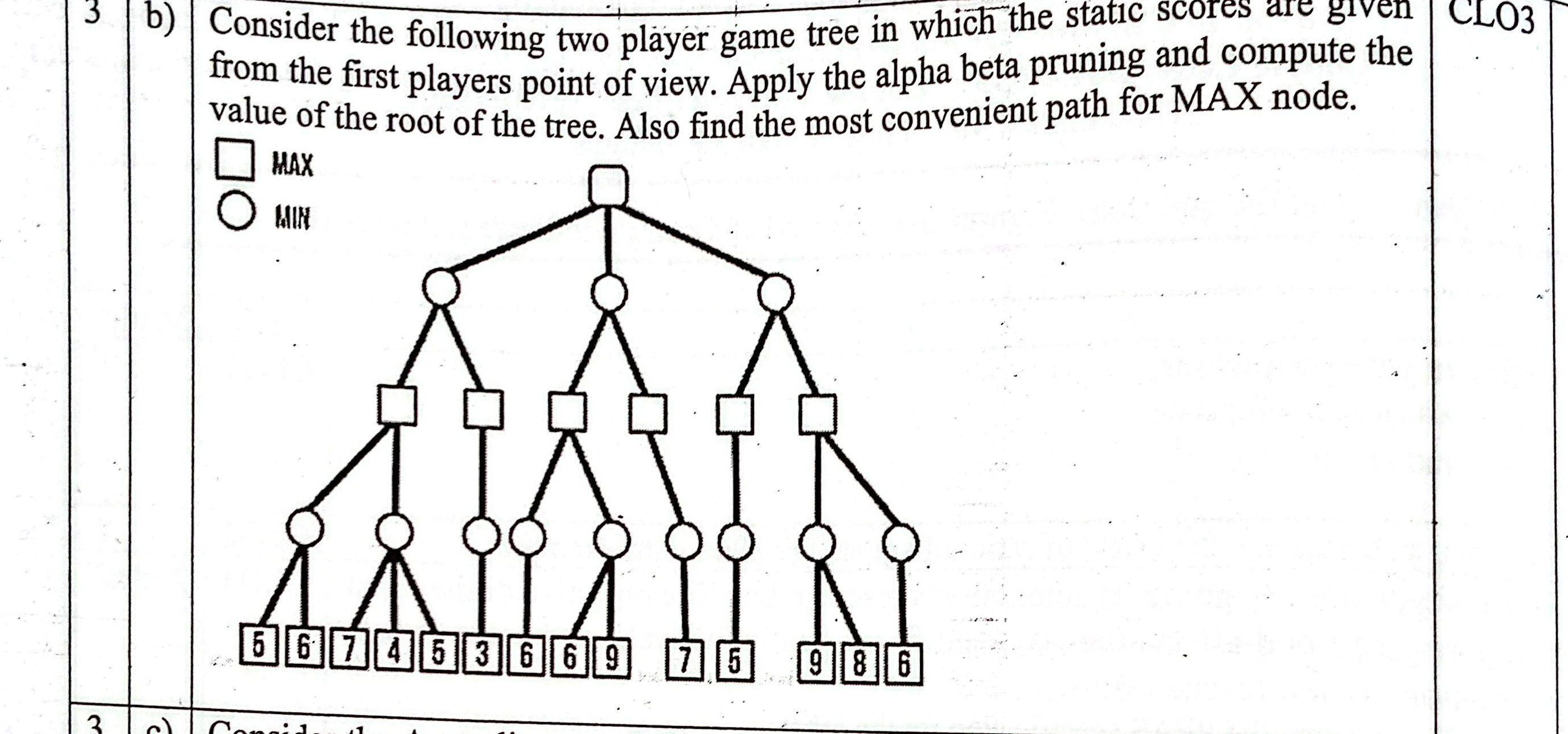
Alpha-Beta Pruning on Two-Player Game Tree:
Tree Structure: Root is MAX node (square). Next layer has 3 MIN nodes (circles: Left \(M_1\), Center \(M_2\), Right \(M_3\)). Layer 3 has MAX nodes, and Layer 4 has terminal static leaf scores.
- Left Subtree (\(M_1\)):
- Left child has leaves \([5, 6]\) → MAX chooses \(\max(5, 6) = 6\).
- Right child has leaves \([7, 4]\) → MAX chooses \(\max(7, 4) = 7\).
- MIN node \(M_1\) chooses \(\min(6, 7) = 6\).
- Root MAX updates: \(\alpha = \max(-\infty, 6) = \mathbf{6}\).
- Center Subtree (\(M_2\)):
- Initial \(\beta = +\infty, \alpha = 6\).
- Left child has leaves \([5, 3]\) → MAX chooses \(\max(5, 3) = 5\).
- MIN node \(M_2\) updates its value: \(\beta = \min(+\infty, 5) = 5\).
- Alpha-Beta Pruning Condition Check: \(\alpha \ge \beta\) (\(6 \ge 5\)).
→ Since MIN already has access to a move yielding 5, it will never allow the outcome to exceed 5. But MAX at the root already has a guaranteed outcome of 6 from the left branch!
→ PRUNING TRIGGERED: The right child of \(M_2\) (with leaves \([6, 6, 9]\)) is COMPLETELY PRUNED!
- Right Subtree (\(M_3\)):
- Initial \(\beta = +\infty, \alpha = 6\).
- Left child has leaves \([7, 5]\) → MAX chooses \(\max(7, 5) = 7\).
- MIN node \(M_3\) updates: \(\beta = \min(+\infty, 7) = 7\).
- Right child has leaves \([9, 8, 6]\) → MAX evaluates leaf 9. Leaf 8 and 6 do not affect maximum (\(\max(9, 8, 6) = 9\)).
- MIN node \(M_3\) chooses \(\min(7, 9) = 7\).
- Root MAX updates: \(\alpha = \max(6, 7) = \mathbf{7}\).
Summary Results:
- Value of the Root Node: \(\mathbf{7}\).
- Pruned Nodes: The entire right subtree of \(M_2\) containing leaves \([6, 6, 9]\).
- Most Convenient Path for MAX Node:
Root (MAX) → Right Branch (M3) → Left MAX Child → Leaf 7.
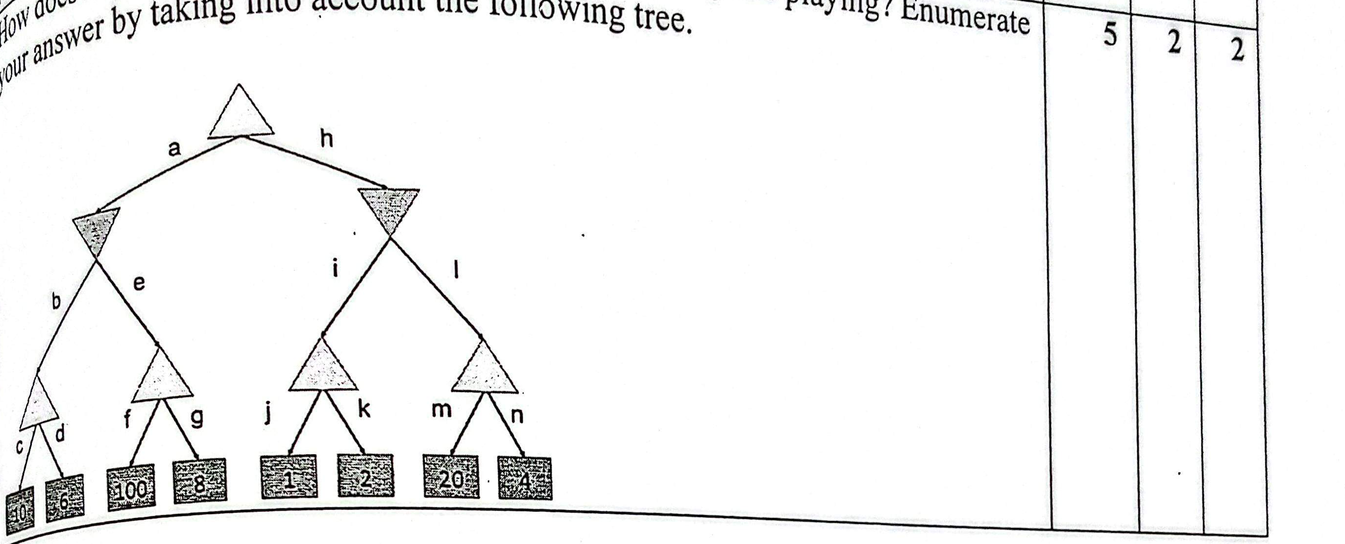
1. How Alpha-Beta Pruning Improves Situation in Game Playing:
Standard Minimax exhaustively searches every leaf node, resulting in exponential time complexity \(O(b^d)\). Alpha-Beta Pruning eliminates branches that cannot possibly influence the final decision of rational players. In the best-case (with optimal move ordering), it cuts the effective branching factor from \(b\) down to \(\sqrt{b}\), reducing time complexity to \(O(b^{d/2})\). This allows the AI agent to search twice as deep in the same amount of computation time.
2. Detailed Evaluation of the Given Game Tree:
Tree: Root \(a\) (MAX). Left branch \(b\) (MIN), Right branch \(h\) (MIN). Under \(b\): \(c\) and \(d\). Under \(h\): \(i\) and \(l\).
- Node \(c\) (MAX): Children are leaves 4 and 6 → \(v(c) = \max(4, 6) = 6\).
- Node \(b\) (MIN): Updates \(\beta = \min(+\infty, 6) = 6\).
- Node \(d\) (MAX): First child evaluated is leaf 100.
→ Since \(d\) is a MAX node, its value is at least 100 (\(v(d) \ge 100\)).
→ Pruning Condition: At node \(b\), \(\beta = 6\). Since child \(d\) has value \(\ge 100\), MIN node \(b\) will never pick \(d\).
→ \(\alpha \ge \beta\) (\(100 \ge 6\)) → Leaf 8 is PRUNED!
→ Value of node \(b = 6\). - Root \(a\) (MAX): Updates \(\alpha = \max(-\infty, 6) = 6\).
- Node \(i\) (MAX): Children are leaves 1 and 2 → \(v(i) = \max(1, 2) = 2\).
- Node \(h\) (MIN): Updates \(\beta = \min(+\infty, 2) = 2\).
→ Pruning Condition: Root \(a\) has \(\alpha = 6\). Node \(h\) has \(\beta = 2\).
→ Since \(\alpha \ge \beta\) (\(6 \ge 2\)), the entire subtree under node \(l\) (containing leaves 20 and 4) is PRUNED!
→ Value of node \(h = 2\). - Root \(a\): Chooses \(\max(6, 2) = \mathbf{6}\).
Summary Table of Node Values & Pruning:
- Node values: \(c = 6\), \(b = 6\), \(a = 6\), \(i = 2\), \(h = 2\).
- Pruned Nodes: Leaf 8 and the entire branch under node \(l\) (leaves 20, 4).
A CSP is formally defined as the triple \(\langle X, D, C angle\): Variables, Domains, Constraints.
| Feature | Standard Search Problem | Constraint Satisfaction Problem (CSP) |
|---|---|---|
| State Representation | Atomic (Black Box): State has no visible internal features. | Factored: State is a set of explicit variable-value assignments. |
| Goal Condition | Evaluated by an arbitrary black-box function GoalTest(s). | Fixed: All variables assigned and all constraints satisfied. |
| Pruning Power | Requires domain-specific heuristics (\(h(n)\)). | Universal domain-independent heuristics: MRV, Degree Heuristic, LCV, AC-3. |
                      AUSTRALIAN MAP TOPOLOGY
                 ┌─────────────────────────────────┐
                 │       Northern Territory (NT)   │───── Queensland (Q)
                 │              /    \             │       /    │
   Western       │             /      \            │      /     │
  Australia (WA)─┤            /        \           │     /      │
                 │           /          \          │    /       │
                 │          /   South    \         │   /   New South
                 │         /   Australia  \────────┼──/    Wales (NSW)
                 │        /      (SA)              │ /          │
                 └───────┴─────────────────────────┴────────────┼───────┐
                                                                │Victoria
                                                                │ (V)
   [ Tasmania (T) ] (Isolated Island)                           └───────┘
- Variables: \(X = \{WA, NT, SA, Q, NSW, V, T\}\)
- Domains: \(D_i = \{\text{Red}, \text{Green}, \text{Blue}\}\)
- Constraints: Adjacent states cannot have identical colors (\(WA e NT, WA e SA, NT e SA, NT e Q, SA e Q, SA e NSW, SA e V, Q e NSW, NSW e V\)). Tasmania \(T\) has no neighbors.
- Step-by-Step Assignment: Assign \(WA = \text{Red} \implies NT \in \{\text{Green}, \text{Blue}\}, SA \in \{\text{Green}, \text{Blue}\}\). Assign \(NT = \text{Green} \implies SA = \mathbf{\text{Blue}}\) (only color left by MRV). \(\implies Q = \mathbf{\text{Red}}, NSW = \mathbf{\text{Green}}, V = \mathbf{\text{Red}}, T = \mathbf{\text{Red}}\).
Yes, this is a CSP.
- Variables: Set of course-section offerings \(X = \{C_1, C_2, \dots, C_k\}\) (e.g.
CSE-3635_SecA). - Domains: Triples \((\text{Classroom } r, \text{Day } d, \text{TimeSlot } t)\) where \(d \in \{\text{Sun, Mon, Tue, Wed, Thu}\}\).
- Hard Constraints:
1. Faculty Clash: Teacher cannot be in two classrooms at the same time.
2. Room Overlap: Two courses cannot occupy the same classroom at the same time.
3. Batch Clash: CSE 5th Sem Sec A cannot have two classes simultaneously.
4. Room Capacity: Room capacity \(\ge\) enrolled students. - Soft Constraints: Minimizing idle gap hours between classes for student batches; faculty preferred teaching days.
| Constraint Filtering Technique | Operational Mechanism | Computational Efficiency & Impact |
|---|---|---|
| Forward Checking | Whenever variable \(X\) is assigned a value, forward checking scans each unassigned neighbor variable \(Y\) connected to \(X\) by a constraint and immediately deletes any value from \(Domain(Y)\) that violates the constraint with \(X\). | Early Failure Detection: If any remaining variable's domain becomes empty (\(\emptyset\)), the algorithm immediately backtracks without branching further. However, it does not look ahead to detect cascade failures between other unassigned variables. |
| Arc Consistency (AC-3 Algorithm) | A directed arc \((X_i \to X_j)\) is arc-consistent if for every value \(x \in Domain(X_i)\), there exists at least one legal value \(y \in Domain(X_j)\) satisfying the binary constraint. AC-3 maintains a queue of all directed arcs in the problem. When a value is removed from \(Domain(X_i)\), all incoming arcs \((X_k \to X_i)\) are re-enqueued for consistency verification. | Global Constraint Propagation: Detects inconsistencies far earlier than forward checking. Runs in \(O(c \cdot d^3)\) time (where \(c\) is number of binary constraints and \(d\) is maximum domain size). Solves many CSPs (like Australian map coloring) with zero backtracking! |

1. Definition of Constraint Satisfaction Problem (CSP):
A Constraint Satisfaction Problem (CSP) is a formal problem representation defined by a 3-tuple \(\langle X, D, C angle\):
- \(X = \{X_1, X_2, \dots, X_n\}\): A finite set of Variables.
- \(D = \{D_1, D_2, \dots, D_n\}\): A set of Domains, where each \(D_i\) specifies the permissible values for \(X_i\).
- \(C = \{C_1, C_2, \dots, C_m\}\): A set of Constraints specifying allowable combinations of variable assignments.
A solution is a complete, consistent assignment of values to all variables that violates zero constraints.
2. Is IIUC CSE Undergraduate Routine Generation an Example of CSP?
YES, absolutely. Timetable scheduling is one of the classic real-world applications of CSP.
Formal Identification of Variables, Domains, and Constraints:
- Variables (\(X\)): Each course section lecture session: $$X = \{L_{c, s, k} \mid c \in \text{Courses (e.g. CSE-3635)}, s \in \text{Sections (e.g. 5A, 5B)}, k \in \text{Weekly Lectures}\}$$
- Domains (\(D\)): Available discrete resource slots: $$D_i = \{ (d, t, r, f) \mid d \in \text{Days (Sun-Thu)}, t \in \text{TimeSlots (8:30-10:00, etc.)}, r \in \text{Rooms}, f \in \text{Faculty} \}$$
- Constraints (\(C\)):
- Hard Constraint 1 (Faculty Clashing): No faculty member can teach two different courses at the same day and time slot: $$\forall i e j, \quad (f_i == f_j \land d_i == d_j) \implies t_i e t_j$$
- Hard Constraint 2 (Student Section Clashing): A student cohort/section cannot attend two classes at the same time: $$\forall i e j, \quad (s_i == s_j \land d_i == d_j) \implies t_i e t_j$$
- Hard Constraint 3 (Room Overbooking): No classroom or laboratory can host two sessions simultaneously: $$\forall i e j, \quad (r_i == r_j \land d_i == d_j) \implies t_i e t_j$$
- Hard Constraint 4 (Room Capacity): \(\text{Capacity}(r_i) \ge \text{EnrolledStudents}(s_i)\).
- Soft Constraints: Minimizing idle gaps between classes for students; honoring preferred teaching time preferences for faculty.

1. Definition of Constraint Satisfaction Problem (CSP):
A Constraint Satisfaction Problem (CSP) is formalized as a triple \(\langle X, D, C angle\):
- Variables \(X\): A set of variables \(\{X_1, X_2, \dots, X_n\}\).
- Domains \(D\): A set of domains \(\{D_1, D_2, \dots, D_n\}\), where \(D_i\) specifies the allowable values for variable \(X_i\).
- Constraints \(C\): A set of constraints \(\{C_1, C_2, \dots, C_m\}\) restricting the combinations of values variables can simultaneously take.
The goal is to find a complete and consistent assignment where every variable is assigned a valid value from its domain without violating any constraints.
2. Differences Between Standard Search-Based Problems and CSP:
| Feature | Standard Search (e.g., Finding Route: City A to City B) | Constraint Satisfaction Problem (CSP) (e.g., Map Coloring) |
|---|---|---|
| State Representation | Atomic / Black Box: A state is just an opaque label (e.g., CurrentNode = City_X). Internal details are invisible to the search algorithm. |
Factored: States are transparent sets of variables and values (e.g., Region_1 = Red, Region_2 = Blue). |
| Goal Test | Domain-Specific: Needs a custom check tailored only to routes (e.g., is_destination(CurrentNode)). |
Universal: Same condition across all CSPs: Every region has a color assigned, and no two adjacent regions share the same color. |
| Heuristics | Hand-Engineered: Must formulate geometry/math specific to navigation (e.g., Euclidean distance or Manhattan distance to the destination). | General-Purpose: Universal strategies like MRV (color the region with the fewest legal colors left) work out of the box without domain knowledge. |
| Inference During Search | Typically None: Expands road segments step-by-step without predicting if a dead-end lies ahead. | Constraint Propagation: When a color is assigned to a region, that color is instantly pruned from the domain of all neighboring regions (via Forward Checking or AC-3). |
| Solution Focus | The Path / Sequence: The exact sequence of turns and road segments taken from start to destination is the actual answer. | The Final State: The final, valid color assignment of the whole map is the only answer; the order in which regions were colored does not matter. |
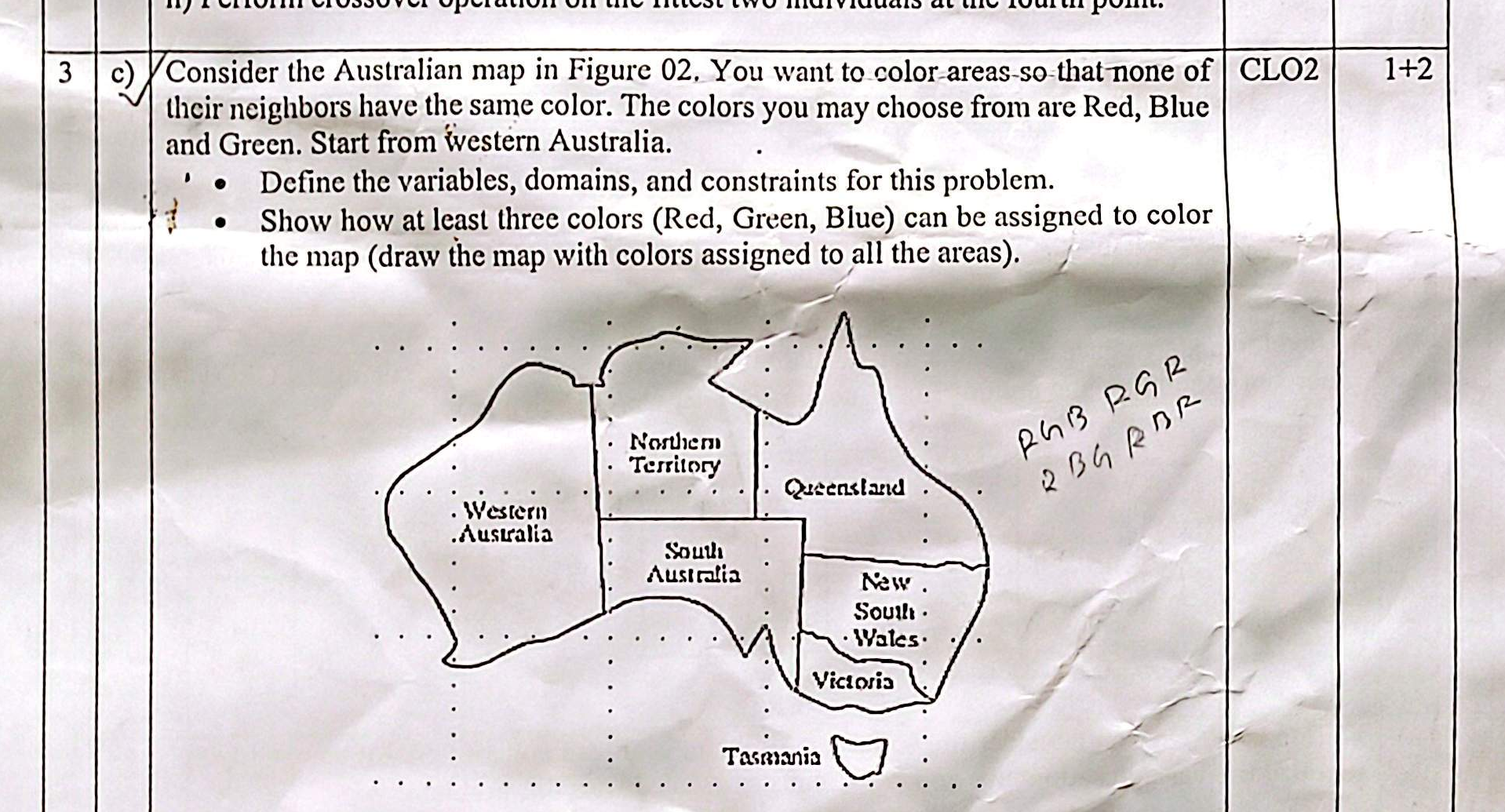
Australian Map Coloring Problem Formulation:
1. Variables (\(X\)): The 7 political territories of Australia:
$$X = \{WA, NT, SA, Q, NSW, V, T\}$$2. Domains (\(D\)): The 3 available colors for each territory:
$$D_i = \{\text{Red, Green, Blue}\} \quad \text{for all } X_i \in X$$3. Constraints (\(C\)): Adjacent regions sharing a land border cannot have the same color:
  WA ≠ NT,   WA ≠ SA,   NT ≠ SA,   NT ≠ Q,
  SA ≠ Q,    SA ≠ NSW,  SA ≠ V,     Q ≠ NSW,   NSW ≠ V
  (Tasmania 'T' has zero land borders with other regions: free variable)
4. Step-by-Step Color Assignment (Starting from Western Australia):
- Assign WA = Red.
- Assign NT = Green (must differ from WA).
- Assign SA = Blue (borders both WA=Red and NT=Green, so Blue is the only valid choice among 3 colors).
- Assign Q = Red (borders NT=Green and SA=Blue).
- Assign NSW = Green (borders SA=Blue and Q=Red).
- Assign V = Red (borders SA=Blue and NSW=Green).
- Assign T = Red (or Green/Blue; completely independent island).
| # | Assigned Variable | Assigned Color | Remaining Valid Domains of Neighbors |
|---|---|---|---|
| 1 | Western Australia (\(WA\)) | Red | \(NT \in \{\text{Green, Blue}\}, \; SA \in \{\text{Green, Blue}\}\) |
| 2 | Northern Territory (\(NT\)) | Green | \(SA \in \{\text{Blue}\}, \; Q \in \{\text{Red, Blue}\}\) |
| 3 | South Australia (\(SA\)) | Blue | \(Q \in \{\text{Red}\}, \; NSW \in \{\text{Red, Green}\}, \; V \in \{\text{Red, Green}\}\) |
| 4 | Queensland (\(Q\)) | Red | \(NSW \in \{\text{Green}\}\) |
| 5 | New South Wales (\(NSW\)) | Green | \(V \in \{\text{Red}\}\) |
| 6 | Victoria (\(V\)) | Red | None |
| 7 | Tasmania (\(T\)) | Red (or Green / Blue) | None (Isolated node) |
Cryptarithmetic is a classical mathematical puzzle in AI where arithmetic operations are encoded using letters of the alphabet. Formulated as a formal CSP:
- Variables: Each unique alphabetic letter in the puzzle.
- Domains: \(D = \{0, 1, 2, 3, 4, 5, 6, 7, 8, 9\}\).
- Unary Constraints: The leading digit of any number cannot be zero (\(\text{Leading Letter} \neq 0\)).
- Global Constraints: \(\text{Alldiff}(X_1, X_2, \dots, X_n)\) — every distinct letter must be mapped to a unique decimal digit.
- Relational Arithmetic Constraints: Column-by-column base-10 summation rules including carries \(c_1, c_2, \dots \in \{0, 1\}\).
            T  O
         +  G  O
        ─────────
         O  U  T
Variables: \(T, O, G, U \in \{0..9\}\). Constraints: \(T \neq 0, G \neq 0, O \neq 0\), all distinct.
- Step 1 (Find O): The sum of two 2-digit numbers is at most \(99 + 99 = 198\). Since the result is a 3-digit number starting with \(O\), the leading carry \(O\) must equal 1.
- Step 2 (Find T): Look at the units column: \(O + O = T \pmod{10}\). Since \(O = 1\): $$1 + 1 = 2 \implies \mathbf{T = 2}$$ There is no carry into the tens column (\(c_1 = 0\)).
- Step 3 (Find G and U): Look at the tens column: \(T + G + c_1 = U + 10 \times O\).
Substituting \(T = 2, c_1 = 0, O = 1\):
$$2 + G = U + 10 \implies G - U = 8$$
Since \(G \le 9\) and \(G, U\) are single digits, the only possible solutions are:
• If \(G = 8 \implies U = 0\). (Valid digits: \(T=2, O=1, G=8, U=0\) — all distinct!).
• If \(G = 9 \implies U = 1\). (Invalid because \(O=1\), violating Alldiff). - Unique Solution: \(\mathbf{T = 2, O = 1, G = 8, U = 0}\).
- Verification: $$\begin{array}{r@{\quad}l} 21 & (TO) \\ +\, 81 & (GO) \\ \hline 102 & (OUT) \end{array}$$ \(\checkmark\) Exactly matches Slide 141!
            S  E  N  D
         +  M  O  R  E
        ───────────────
         M  O  N  E  Y
Variables: \(S, E, N, D, M, O, R, Y \in \{0..9\}\). Constraints: \(S \neq 0, M \neq 0\), all distinct.
- Step 1 (Find M): The sum of two 4-digit numbers can generate at most a carry of 1 into the 5th column. Therefore, \(M = 1\).
- Step 2 (Find O and S): Look at the thousands column: \(S + M + c_3 = O + 10 \times M\). $$S + 1 + c_3 = O + 10 \implies S + c_3 = O + 9$$ Since \(S \le 9\) and \(c_3 \le 1\), the left side is at most \(10\). Thus \(O\) can only be \(0\) or \(1\). But \(M = 1\), and all letters must be distinct, so \(O = 0\). With \(O = 0\): \(S + c_3 = 9\). If \(c_3 = 0\), then \(S = 9\). (If \(c_3 = 1\), then \(S = 8\); we will see below that a carry into column 4 must occur, so \(S = 9\) and \(c_3 = 0\)).
- Step 3 (Find E and N): Look at the hundreds column: \(E + O + c_2 = N + 10 \times c_3\). Since \(O = 0\) and \(c_3 = 0\): \(E + c_2 = N\). Since all letters are distinct, \(E \neq N\), which forces carry \(c_2 = 1\), meaning: $$\mathbf{N = E + 1}$$
- Step 4 (Find R): Look at the tens column: \(N + R + c_1 = E + 10 \times c_2\). Substitute \(N = E + 1\) and \(c_2 = 1\): $$(E + 1) + R + c_1 = E + 10 \implies R + c_1 = 9$$ If \(c_1 = 0\), then \(R = 9\). But \(S = 9\), so \(R\) cannot be 9. Therefore, \(c_1 = 1\) and \(R = 8\).
- Step 5 (Find D, E, Y): Look at the units column: \(D + E = Y + 10 \times c_1 = Y + 10\) (since \(c_1 = 1\)).
We need \(D + E \ge 12\). The remaining available unused digits from \(\{0, 1, 2, 3, 4, 5, 6, 7, 8, 9\}\) are \(\{2, 3, 4, 5, 6, 7\}\) (since 0, 1, 8, 9 are already assigned).
• If \(E = 5 \implies N = E + 1 = 6\).
• Then \(D + 5 = Y + 10 \implies D = Y + 5\).
• With available digits, choosing \(\mathbf{D = 7}\) gives \(\mathbf{Y = 2}\)! - Final Unique Assignment: $$\mathbf{S = 9,\; E = 5,\; N = 6,\; D = 7,\; M = 1,\; O = 0,\; R = 8,\; Y = 2}$$
- Verification: $$\begin{array}{r@{\quad}l} 9567 & (SEND) \\ +\, 1085 & (MORE) \\ \hline 10652 & (MONEY) \end{array}$$ \(\checkmark\) Exactly matches Slide 142!
| Slide Puzzle | Cryptarithmetic Layout | Digit Mapping Solution | Arithmetic Verification |
|---|---|---|---|
| Puzzle 3 (Slide 143): EAT + THAT = APPLE |
    E A T
+ T H A T
─────────
A P P L E
|
\(\mathbf{E = 8}\) \(\mathbf{A = 1}\) \(\mathbf{T = 9}\) \(\mathbf{H = 2}\) \(\mathbf{P = 0}\) \(\mathbf{L = 3}\) |
$$\begin{array}{r@{\quad}l} 819 & (EAT) \\ +\, 9219 & (THAT) \\ \hline 10038 & (APPLE) \end{array}$$
• \(T+T = 9+9 = 18 \implies E=8, c_1=1\) • \(A+A+1 = 1+1+1 = 3 \implies L=3, c_2=0\) • \(E+H = 8+2 = 10 \implies P=0, c_3=1\) • \(T+1 = 9+1 = 10 \implies AP = 10\). \(\checkmark\) |
| Puzzle 4 (Slide 143): SOME + TIME = SPENT |
  S O M E
+ T I M E
─────────
S P E N T
|
\(\mathbf{S = 1}\) \(\mathbf{O = 9}\) \(\mathbf{M = 3}\) \(\mathbf{E = 4}\) \(\mathbf{T = 8}\) \(\mathbf{I = 5}\) \(\mathbf{P = 0}\) \(\mathbf{N = 6}\) |
$$\begin{array}{r@{\quad}l} 1934 & (SOME) \\ +\, 8534 & (TIME) \\ \hline 10468 & (SPENT) \end{array}$$
• \(E+E = 4+4 = 8 \implies T=8, c_1=0\) • \(M+M = 3+3 = 6 \implies N=6, c_2=0\) • \(O+I = 9+5 = 14 \implies E=4, c_3=1\) • \(S+T+1 = 1+8+1 = 10 \implies SP = 10\). \(\checkmark\) |
| Puzzle 5 (Slide 143): BASE + BALL = GAMES |
  B A S E
+ B A L L
─────────
G A M E S
|
\(\mathbf{B = 7}\) \(\mathbf{A = 4}\) \(\mathbf{S = 8}\) \(\mathbf{E = 3}\) \(\mathbf{L = 5}\) \(\mathbf{G = 1}\) \(\mathbf{M = 9}\) |
$$\begin{array}{r@{\quad}l} 7483 & (BASE) \\ +\, 7455 & (BALL) \\ \hline 14938 & (GAMES) \end{array}$$
• \(E+L = 3+5 = 8 \implies S=8, c_1=0\) • \(S+L = 8+5 = 13 \implies E=3, c_2=1\) • \(A+A+1 = 4+4+1 = 9 \implies M=9, c_3=0\) • \(B+B = 7+7 = 14 \implies GA = 14\). \(\checkmark\) |
Branch and Bound (Uniform Cost Search) finds the lowest-cost path from the start node (\(S\)) to the goal node (\(G\)):
- Branch: Expand paths one step at a time.
- Bound: Always pick the path with the lowest total accumulated cost so far. Any path whose cost exceeds the best complete path to \(G\) is pruned (discarded).
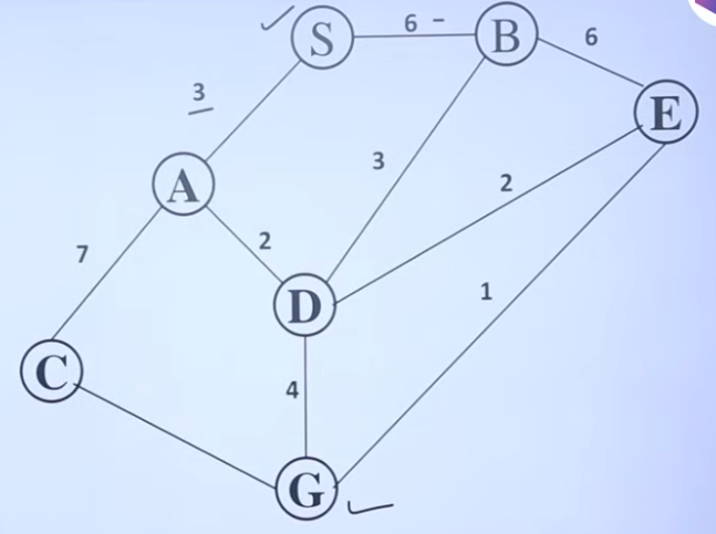
Step 1: Start at \(S\)
Paths from \(S\):
- \(S \to A = 3\)
- \(S \to B = 6\)
Priority Queue: [ (S-A: 3), (S-B: 6) ]
Step 2: Expand the lowest-cost path (\(S \to A\))
From \(A\), explore neighbors (excluding \(S\)):
- \(S \to A \to D = 3 + 2 = 5\)
- \(S \to A \to C = 3 + 7 = 10\)
Priority Queue: [ (S-A-D: 5), (S-B: 6), (S-A-C: 10) ]
Step 3: Expand the lowest-cost path (\(S \to A \to D\))
From \(D\), explore unvisited neighbors:
- \(S \to A \to D \to E = 5 + 2 = 7\)
- \(S \to A \to D \to B = 5 + 3 = 8\)
- \(S \to A \to D \to G = 5 + 4 = 9\) (First complete path to Goal)
Priority Queue: [ (S-B: 6), (S-A-D-E: 7), (S-A-D-B: 8), (S-A-D-G: 9), (S-A-C: 10) ]
Step 4: Expand the lowest-cost path (\(S \to B\))
From \(B\), explore unvisited neighbors:
- \(S \to B \to D = 6 + 3 = 9\)
- \(S \to B \to E = 6 + 6 = 12\)
Priority Queue: [ (S-A-D-E: 7), (S-A-D-B: 8), (S-A-D-G: 9), (S-B-D: 9), (S-A-C: 10), (S-B-E: 12) ]
Step 5: Expand the lowest-cost path (\(S \to A \to D \to E\))
From \(E\), explore neighbor \(G\):
- \(S \to A \to D \to E \to G = 7 + 1 = \mathbf{8}\)
Priority Queue: [ (S-A-D-E-G: 8), (S-A-D-B: 8), (S-A-D-G: 9), (S-B-D: 9), (S-A-C: 10), (S-B-E: 12) ]
Step 6: Goal Selection & Bounding (Pruning)
The minimum cost in the queue is now 8 for the path \(S \to A \to D \to E \to G\).
Because this path reaches the Goal \(G\) with cost 8, all remaining open paths with cost \(\ge 8\) (such as \(S \to A \to C\) which already costs 10) are bounded and pruned without further expansion.
Optimal Solution:
- Optimal Path: \(S \to A \to D \to E \to G\)
- Minimum Cost: \(\mathbf{8}\)
Branch and Bound (B&B) is an exact algorithmic paradigm designed to find optimal solutions to NP-hard discrete combinatorial optimization problems (such as the Travelling Salesman Problem, 0/1 Knapsack, and Job-Shop Scheduling) without exhaustive brute-force search.
| Component | Algorithmic Mechanism | Purpose & Impact |
|---|---|---|
| 1. Branching | Recursively partitions the search space into smaller mutually exclusive subproblems (children nodes) representing partial solution assignments. | Builds a state-space tree of candidate solutions. |
| 2. Bounding | Calculates an estimated mathematical bound on the best possible objective function value achievable by expanding any completion of the partial node:
• Lower Bound (LB) for Minimization problems (e.g. TSP tour cost). • Upper Bound (UB) for Maximization problems (e.g. Knapsack profit). |
Provides a rigorous mathematical ceiling/floor for whole subtrees without exploring them. |
| 3. Pruning | If a node's bound is worse than the best known feasible solution found so far (the incumbent solution), that node is immediately pruned (killed). | Dramatically shrinks the search space, rendering computationally intractable problems solvable in practice. |
| 4. Search Strategies | Explores the state space tree using:
• Best-First Search (LCBB): Uses a priority queue to expand the most promising bound first. • FIFO / Breadth-First: Explores level by level. • LIFO / Depth-First: Rapidly descends to find an early incumbent solution. |
Determines how quickly tight bounds and optimal solutions are discovered. |
Consider the complete undirected weighted graph from the course lecture slide with 5 vertices \(\{0, 1, 2, 3, 4\}\):
                                  (1)
                                3/ | \1
                                /  |4 \
                               /   |   (2)
                             (0)   |   /2
                             8\ \7 |  /
                               \ \ | /
                                \  (3)
                               3 \ /
                                 (4)
| Edge | Weight | Edge | Weight | Edge | Weight |
|---|---|---|---|---|---|
(0, 1) | 3 | (1, 2) | 1 | (2, 3) | 2 |
(0, 3) | 7 | (1, 3) | 4 | (3, 4) | 3 |
(0, 4) | 8 | — | — | — | — |
Goal: Find a simple cycle that visits every vertex \(\{0, 1, 2, 3, 4\}\) exactly once and returns to the start vertex with minimum total edge weight.
Bounding Mechanism (Sum of 2 Cheapest Incident Edges): For each vertex \(v\), any valid Hamiltonian tour must enter and leave \(v\) through two distinct incident edges. Hence, a rigorous Lower Bound on any complete tour is:
$$\text{Lower Bound} = \frac{1}{2} \sum_{v \in V} \left( \text{cost of cheapest edge incident to } v + \text{cost of 2nd cheapest edge incident to } v \right)$$- Vertex 0: incident weights are 3, 7, 8 \(\implies\) two cheapest are \(3 + 7 = 10\).
- Vertex 1: incident weights are 1, 3, 4 \(\implies\) two cheapest are \(1 + 3 = 4\).
- Vertex 2: incident weights are 1, 2 \(\implies\) two cheapest are \(1 + 2 = 3\).
- Vertex 3: incident weights are 2, 3, 4, 7 \(\implies\) two cheapest are \(2 + 3 = 5\).
- Vertex 4: incident weights are 3, 8 \(\implies\) two cheapest are \(3 + 8 = 11\).
Branching: Construct candidate tours starting at vertex 0:
• Tour \(0 \to 1 \to 2 \to 3 \to 4 \to 0\):
$$\text{Cost} = c(0,1) + c(1,2) + c(2,3) + c(3,4) + c(4,0) = 3 + 1 + 2 + 3 + 8 = \mathbf{17}!$$
Because the actual tour cost (\(17\)) exactly matches the theoretical minimum lower bound ceiling, this tour is provably optimal! All other branches exceeding 17 are pruned immediately without expansion.
Consider the 0/1 Knapsack problem instance with knapsack capacity \(W_{\max} = 12\):
Sorted in decreasing order of greedy efficiency (decision order):
| Decision Order (\(k\)) | Original Item (\(i\)) | Profit (\(P\)) | Weight (\(W\)) | Ratio (\(P/W\)) |
|---|---|---|---|---|
| 1 | Item 4 | 24 | 2 | \(\mathbf{12}\) |
| 2 | Item 1 | 30 | 5 | \(\mathbf{6}\) |
| 3 | Item 3 | 20 | 4 | \(\mathbf{5}\) |
| 4 | Item 2 | 28 | 7 | \(\mathbf{4}\) |
At any node with current weight \(cw\) and current profit \(cp\):
- If \(cw > 12\): Infeasible (Pruned immediately).
- Otherwise, calculate Upper Bound (\(UB\)) by continuous fractional relaxation:
Level 0: Root Node
\(cw = 0, cp = 0\)
Fill knapsack capacity (12):
- Take Item 4: weight \(2 \implies cp = 24\), remaining capacity \(= 10\)
- Take Item 1: weight \(5 \implies cp = 54\), remaining capacity \(= 5\)
- Take Item 3: weight \(4 \implies cp = 74\), remaining capacity \(= 1\)
- Take fraction of Item 2: \(\frac{1}{7} \times 28 = 4\)
Root \(UB\) \(= 74 + 4 = \mathbf{78}\)
Level 1: Decide on Item 4 (\(P=24, W=2\))
-
Branch Left (\(x_4 = 1\)):
\(cw = 2\), \(cp = 24\). Remaining capacity \(= 10\).
Greedy fill: Item 1 (full, 30) + Item 3 (full, 20) + fraction of Item 2 (\(\frac{1}{7} \times 28 = 4\)).
$$UB = 24 + 30 + 20 + \frac{1}{7}(28) = \mathbf{78}$$ -
Branch Right (\(x_4 = 0\)):
\(cw = 0\), \(cp = 0\). Remaining capacity \(= 12\).
Greedy fill: Item 1 (\(W=5, P=30\)) + Item 3 (\(W=4, P=20\)) + fraction of Item 2 (\(\frac{3}{7} \times 28 = 12\)).
$$UB = 0 + 30 + 20 + 12 = \mathbf{62}$$
Level 2: Decide on Item 1 (\(P=30, W=5\))
Expand best active node: \((x_4 = 1, UB = 78)\)
-
Branch Left (\(x_1 = 1\)):
\(cw = 2 + 5 = 7\), \(cp = 24 + 30 = 54\). Remaining capacity \(= 12 - 7 = 5\).
Greedy fill: full Item 3 (\(W=4, P=20\)) + fraction of Item 2 (\(\frac{1}{7} \times 28 = 4\)).
$$UB = 54 + 20 + 4 = \mathbf{78}$$ -
Branch Right (\(x_1 = 0\)):
\(cw = 2\), \(cp = 24\). Remaining capacity \(= 10\).
Greedy fill: full Item 3 (\(W=4, P=20\)) + fraction of Item 2 (\(\frac{6}{7} \times 28 = 24\)).
$$UB = 24 + 20 + 24 = \mathbf{68}$$
Level 3: Decide on Item 3 (\(P=20, W=4\))
Expand best active node: \((x_4 = 1, x_1 = 1, UB = 78)\)
-
Branch Left (\(x_3 = 1\)):
\(cw = 7 + 4 = 11\), \(cp = 54 + 20 = 74\). Remaining capacity \(= 12 - 11 = 1\).
Greedy fill: fraction of Item 2 (\(\frac{1}{7} \times 28 = 4\)).
$$UB = 74 + 4 = \mathbf{78}$$ -
Branch Right (\(x_3 = 0\)):
\(cw = 7\), \(cp = 54\). Remaining capacity \(= 5\).
Greedy fill: fraction of Item 2 (\(\frac{5}{7} \times 28 = 20\)).
$$UB = 54 + 20 = \mathbf{74}$$
Level 4: Decide on Item 2 (\(P=28, W=7\))
Expand best active node: \((x_4 = 1, x_1 = 1, x_3 = 1, UB = 78)\)
-
Branch Left (\(x_2 = 1\)):
\(cw = 11 + 7 = 18 > 12 \implies\) ❌ Pruned (Exceeds capacity) -
Branch Right (\(x_2 = 0\)):
\(cw = 11 \le 12\), \(cp = \mathbf{74}\).
Leaf reached: Current Best Solution (\(\text{Incumbent}\)) = 74.
Level 5: Pruning Remaining Open Branches
Check the remaining open nodes in the priority queue against incumbent (\(\text{Best} = 74\)):
- Node \((x_4=1, x_1=1, x_3=0)\) has \(UB = 74 \le 74 \implies\) Pruned
- Node \((x_4=1, x_1=0)\) has \(UB = 68 < 74 \implies\) Pruned
- Node \((x_4=0)\) has \(UB = 62 < 74 \implies\) Pruned
All other branches are pruned because their maximum possible yield cannot exceed 74.
                     [ Root ]
                     (UB = 78)
                     /       \
               x₄=1 /         \ x₄=0
                   /           \
           (cw=2, cp=24)      (UB = 62) [Pruned < 74]
             UB = 78
             /     \
       x₁=1 /       \ x₁=0
           /         \
   (cw=7, cp=54)    (UB = 68) [Pruned < 74]
     UB = 78
     /     \
x₃=1/       \ x₃=0
   /         \
(cw=11, cp=74) (UB = 74) [Pruned ≤ 74]
  UB = 78
  /     \
x₂=1     x₂=0
 |        |
cw=18    (cw=11, cp=74)  <-- ★ OPTIMAL SOLUTION
> 12
(Pruned)
Final Result:
- Selected Items: Item 4, Item 1, and Item 3 (\(x_4=1, x_1=1, x_3=1, x_2=0\))
- Total Weight: \(2 + 5 + 4 = \mathbf{11} \le 12\)
- Maximum Profit: \(24 + 30 + 20 = \mathbf{74}\)
Problem Reduction: A problem-solving method where a complex goal is recursively decomposed into smaller, simpler sub-problems until primitive, easily solvable tasks are reached.
AND Nodes: Represent decomposition (all child components must be accomplished). OR Nodes: Represent alternatives (solving any one child suffices).
                              [ Produce & Publish IIUC Vlog ]
                                             │
                       ┌─────────────────────┴─────────────────────┐
                       │                   ( AND Arc )             │
                       ▼                         ▼                 ▼
             [ Content Creation ]       [ Video Production ] [ Publication & Outreach ]
                     │                           │                         │
         ┌───────────┴───────────┐         ┌─────┴─────┐             ┌─────┴─────┐
         │ (AND)                 │         │ (AND)     │             │ (AND)     │
         ▼                       ▼         ▼           ▼             ▼           ▼
    [ Scriptwriting ]     [ Interview ] [ Footage ] [ Audio ]     [ IIUC Media] [ Student Club]
         │                 Segments     Capture     Voiceover      Web/Portal   Distribution
    ┌────┴────┐                  │         │           │             │                 │
    ▼         ▼                  ▼      ┌──┴──┐     ┌──┴──┐       ┌──┴──┐           ┌──┴──┐
 [Student  [Teacher          [Fest    [Drone [DSLR] [Studio [Phone[IIUC  [Official  [WhatsApp[Facebook
  Inter-    Quotes]         Schedule] Camera]        Mic]   Mic]   Site]  YouTube]   Groups]   Groups]
  views]                        (OR)    (OR)        (OR)           (OR)               (OR)

1. What is the Problem Reduction Technique in AI?
Problem Reduction is an algorithmic problem-solving strategy that decomposes a complex, high-level goal problem into a hierarchy of smaller, manageable subproblems. A solution to the overall problem is achieved when a sufficient set of subproblems are solved. It is mathematically formalized and searched using AND-OR Graphs and the AO* search algorithm.
2. AND-OR Graph Modeling for IIUC Tech Fest 2026 Promotional Vlog:
                                [Produce & Publish IIUC Vlog]
                                           |  (AND Arc)
            +------------------------------+------------------------------+
            |                                                             |
   [Video Production]                                            [Audio Production]
            | (AND Arc)                                                   | (OR Branch)
    +-------+-------+                                             +-------+-------+
    |       |       |                                             |               |
 [Script] [Shoot] [Edit]                                      [Voiceover]     [Tech BGM]
            |
            | (AND)
   [Distribute to Community]
            | (OR Branch)
    +-------+-------+
    |       |       |
[IIUC FB] [CSE YT] [Campus LEDs]
Explanation of Nodes:
- Root Goal (AND node):
Produce & Publish IIUC Vlogrequires ALL THREE of:Video ProductionANDAudio ProductionANDDistribution to Community. - Video Production (AND node): Requires
ScriptingANDCampus Footage ShootingANDVideo Editing. - Audio Production (OR node): Can be satisfied by either
Student Voiceover NarrationORLicensing Tech Background Music. - Distribution (OR node): Can be published on either
IIUC Official Facebook PageORIIUC CSE YouTube ChannelORCampus Digital Display LEDs.